Table of contents
(2023-11-22)
Discrete Convolve
Source video: 【官方双语】那么……什么是卷积?- 3B1B
-
Two list of numbers are combined and form a new list: Make a table, calculate pairwise product for each cell and sum up all anti-diagonals.
$(a * b)\_n = ∑_{\substack{i,j \\\ i+j=n}} a_i * b_j$
- The sum of indecies of the 2 number in each pair to be summed up is the same, just distinct combinations.
-
Reverse the second list, slide it from left to righ, and sum the products of each pair aligned vertically.
-
Convolution for image is for smoothing by averaging nearby pixels.
-
The multiplication of two polynomials is convolution, because multiply each two term and collect term with the same order.
-
(2024-01-12) 父亲寿命 和 儿子的年龄做卷积,等于一起生活的岁月
(2023-11-07)
Covariance Matrix is PSD
-
Variance is the average of the squared distance between the mean and point for a single dimension.
方差是偏离期望的平方的期望。
$$Var(x) = \frac{∑(x-μ)²}{n}$$Variance is a scalar: the averaged squared mangitude of the distance vector between a certain vector and the mean vector in a data space. -
Covariance is the product of 2 distances betwee mean and point for the 2 dimensions respectively.
$$Covar(x,y) = \frac{∑(x-μ_x)(y-μ_y)}{n}$$Covariance is a real number and indicates positive- or negtive correlation of 2 dimensions by its sign.
-
Covariance matrix is a symmatric matrix recording covariance for each pair of dimensions.
$$ \begin{array}{c|ccc} 𝐱 & d₁ & d₂ & d₃ \\\ \hline \\\ d₁ & \frac{∑(x_{d₁}-μ_{d₁})(x_{d₁}-μ_{d₁})}{n} & \frac{∑(x_{d₁}-μ_{d₁})(x_{d₂}-μ_{d₂})}{n} & \frac{∑(x_{d₁}-μ_{d₁})(x_{d₃}-μ_{d₃})}{n} \\\ \\\ d₂ & \frac{∑(x_{d₂}-μ_{d₂})(x_{d₁}-μ_{d₁})}{n} & \frac{∑(x_{d₂}-μ_{d₂})(x_{d₂}-μ_{d₂})}{n} & \frac{∑(x_{d₂}-μ_{d₂})(x_{d₃}-μ_{d₃})}{n} \\\ \\\ d₃ & \frac{∑(x_{d₃}-μ_{d₃})(x_{d₁}-μ_{d₁})}{n} & \frac{∑(x_{d₃}-μ_{d₃})(x_{d₂}-μ_{d₂})}{n} & \frac{∑(x_{d₃}-μ_{d₃})(x_{d₃}-μ_{d₃})}{n} \end{array} $$Thus, element on the main diagonal is the variance of each variable.
-
Covariance matrix is always positive semi-definite, symmetric, square.
-
The eigenvalues λ and eigenvectors 𝐯 of covariance matrix 𝐄(𝐱𝐱ᵀ) can be solved from:
𝐄(𝐱𝐱ᵀ) ⋅ 𝐯 = λ𝐯
Since 𝐄(𝐱𝐱ᵀ) is a symmetric matrix, λs are all real numbers.
-
λ = 𝐄(𝐱𝐱ᵀ) = $\frac{∑(xᵢ-μᵢ)²}{n}$ ≥ 0,
where n is the number of datapoints in the dataset. xᵢ is one of dimensions of 𝐱. xᵢ is a column vector containing n points.
-
Check the definition of positive semi-definite:
𝐯ᵀ𝐄 𝐯 = λ𝐯ᵀ𝐯 = λ[a b c] $[^a\_{^b\_c}]$ = λ(a²+b²+c²) ≥ 0.
Thus, covariance matrix 𝐄 is positive semi-definite.
todo: This could be wrong, need to watch Dr. Strang’s lecture.
The following proof is from Is a sample covariance matrix always symmetric and positive definite? - SE
-
Covariance matrix E(𝐱𝐱ᵀ) = (𝐱-𝛍)(𝐱-𝛍)ᵀ/n
-
Check the definition of positive semi-definite:
𝐯ᵀ E(𝐱𝐱ᵀ) 𝐯 = $\frac{1}{n}$ 𝐯ᵀ (𝐱-𝛍)(𝐱-𝛍)ᵀ 𝐯 = ((𝐱-𝛍)ᵀ 𝐯)²/n ≥ 0. A positive scalar.
Other Proofs:
-
-
Since covariance matrix is positive semi-definite, there is global minima for all axis:
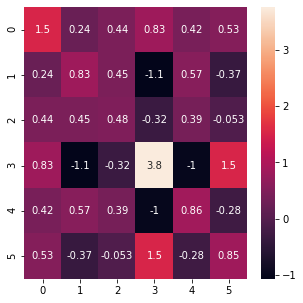
Heatmap of a covariance matrix - Gowri Shankar
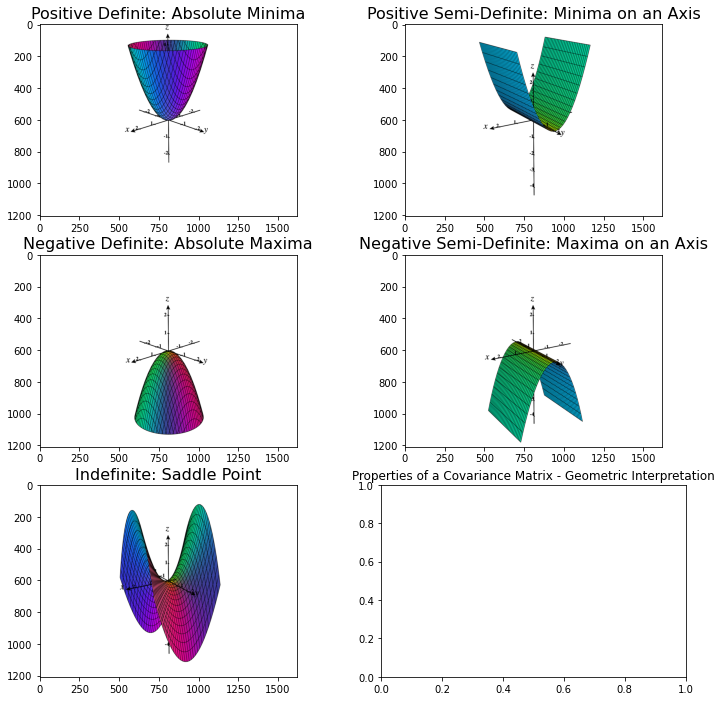
Categorizing Quadratic Forms - Ximera, OSU - Categorizing Quadratic Forms
(2023-11-08)
Radius of 3D Gaussian
If a dataset scattered as an ellipse following 2D Gaussian is circumscribed by a circle, to cover the most points, the radius of the circle could be $r = 3σ$, 3 times the standard deviation.

The standard deviation σ is the square root of the variance, which is the element on the main diagonal of the covariance matrix.
And variances are the eigenvalues of the covariance matrix.
Given a covariance matrix $𝐂=[^{a \ b}_{b \ c}]$, its eigenvalue λ and eigenvector 𝐯 satisfy: 𝐂 𝐯 = λ𝐯.
Eigenvalues λs can be solved from: $\rm det(𝐂 - λ𝐈) = 0$:
$$ \begin{vmatrix} a-λ & b \\\ b & c-λ\end{vmatrix} = 0 \\\ (a-λ)(c-λ) - b^2 = 0 \\\ λ^2 - (a+c)λ + ac-b^2 =0 $$λ₁ = $\frac{(a+c) + \sqrt{(a+c)^2 - 4(ac-b^2)} }{2}$, λ₂ = $\frac{(a+c) - \sqrt{(a+c)^2 - 4(ac-b^2)} }{2}$