3 线性判别分析 (Fisher判别分析) - 模型定义

Source Video-P3

Data:

$$ \begin{aligned} \text{Samples:}\ & \mathbf X = (\mathbf x_1, \mathbf x_2, \cdots, \mathbf x_N)^T_{N\times p} = \begin{pmatrix} \mathbf x_1^T \ \mathbf x_2^T \ \vdots \ \mathbf x_N^T \end{pmatrix}_{N \times p} \\

\text{Samples:} \ & \mathbf Y = \begin{pmatrix} y_1 \ y_2 \ \vdots \ y_N \end{pmatrix}_{N \times 1} \\

\text{Abbreviations:}\ & \left{ (\mathbf x_i, y_i) \right}_{i=1}^N, \ \mathbf x_i \in \R^p, \ \underset{(\text{2class: } C_1,C_2)}{y_i \in {+1, -1}}\\

\text{2 Group:}\ &\mathbf x_{C_1} = { \mathbf x_i | y_i=+1} ; \quad \mathbf x_{C_2} = { \mathbf x_i | y_i=-1} \\

\text{Number:}\ & |\mathbf x_{C_1}| = N_1, \ |\mathbf x_{C_2}|=N_2, \ N_1 + N_2 = N \end{aligned} $$

Fisher

• 类内小，类间大

• 把p维降到1维，投影到某一个轴上再做分类。
  在投影方向($\mathbf w$)上，类内点的坐标方差足够小，类间距离要大
  投影方向就是分类超平面（$\mathbf w^T \mathbf x$）的法向量。

• 记号

  限定 $\| \mathbf w \| =1$

  样本点$\mathbf x_i$ 在投影轴$\mathbf w$上的投影长度: $z_i = \mathbf w^T \mathbf x_i$

  $$ \begin{aligned}

  均值: \overline{z} =& \frac{1}{N} \sum_{i=1}^N z_i = \frac{1}{N} \sum_{i=1}^N \mathbf w^T \mathbf x_i \

  协方差矩阵: S_{z} =& \frac{1}{N} \sum_{i=1}^N (z-\overline z)(z-\overline z)^T \

  =& \frac{1}{N} \sum_{i=1}^N (\mathbf w^T \mathbf x_i-\overline z)(\mathbf w^T \mathbf x_i-\overline z)^T \

  类C_1:\ \overline{z_1} =& \frac{1}{N_1} \sum_{i=1}^{N_1} \mathbf w^T \mathbf x_i \

    S_{z_1} =&\frac{1}{N_1} \sum_{i=1}^{N_1} (\mathbf w^T \mathbf x_i-\overline{z_1})(\mathbf w^T \mathbf x_i-\overline{z_1})^T \\
  

  类C_2:\ \overline{z_2} =& \frac{1}{N_2} \sum_{i=1}^{N_1} \mathbf w^T \mathbf x_i \

    S_{z_2} =& \frac{1}{N_2} \sum_{i=1}^{N_2} (\mathbf w^T \mathbf x_i-\overline{z_2})(\mathbf w^T \mathbf x_i-\overline{z_2})^T \\
  

  类内距离: & S_{z_1} + S_{z_2} \ 类间距离: & (\overline{z_1} - \overline{z_2})^2 \

  目标函数: & J(\mathbf w) = \frac{(\overline{z_1} - \overline{z_2})^2}{S_{z_1} + S_{z_2}} \

  分子：& \left[ \frac{1}{N_1} \sum_{i=1}^{N_1} \mathbf w^T \mathbf x_i-\frac{1}{N_2} \sum_{i=1}^{N_1} \mathbf w^T \mathbf x_i \right]^2 \

    =& \left[ \mathbf w^T \left( \frac{1}{N_1} \sum_{i=1}^{N_1}\mathbf x_i-\frac{1}{N_2} \sum_{i=1}^{N_1} \mathbf x_i \right) \right]^2\\
  
    =& \left[ \mathbf w^T (\overline{\mathbf x_{C_1}}-\overline{\mathbf x_{C_2}}) \right]^2\\
    =& \mathbf w^T (\overline{\mathbf x_{C_1}}-\overline{\mathbf x_{C_2}}) (\overline{\mathbf x_{C_1}}-\overline{\mathbf x_{C_2}})^T \mathbf w^T \\ 
  

  S_{z_1}=& \frac{1}{N_1} \sum_{i=1}^{N_1} (\mathbf w^T \mathbf x_i - \frac{1}{N_1} \sum_{j=1}^{N_1} \mathbf w^T \mathbf x_j)(\mathbf w^T \mathbf x_i - \frac{1}{N_1} \sum_{j=1}^{N_1} \mathbf w^T \mathbf x_j)^T \

    =& \frac{1}{N_1}\sum_{i=1}^{N_1} \mathbf w^T (\mathbf x_i - \overline{\mathbf x_{C_1}}) (\mathbf x_i - \overline{\mathbf x_{C_1}})^T \mathbf w\\
  
    =& \mathbf w^T \left[ \frac{1}{N}\sum_{i=1}^{N_1}  (\mathbf x_i - \overline{\mathbf x_{C_1}}) (\mathbf x_i - \overline{\mathbf x_{C_1}})^T \right] \mathbf w \\
  
    =& \mathbf w^T S_{C_1} \mathbf w \\
  

  分母：& \mathbf w^T S_{C_1} \mathbf w + \mathbf w^T S_{C_2} \mathbf w\ =& \mathbf w^T (S_{C_1} + S_{C_2}) \mathbf w \

  J(\mathbf w) =& \frac{\mathbf w^T (\overline{\mathbf x_{C_1}}-\overline{\mathbf x_{C_2}}) (\overline{\mathbf x_{C_1}}-\overline{\mathbf x_{C_2}})^T \mathbf w^T} {\mathbf w^T (S_{C_1} + S_{C_2}) \mathbf w} \ =& \frac{\mathbf w^T S_b \mathbf w}{\mathbf w^T S_{w} \mathbf w} \quad \text{($S_b$: 类间方差; $S_w$: 类内方差)} \ =& \mathbf w^T S_b \mathbf w \cdot (\mathbf w^T S_{w} \mathbf w)^{-1}

  \end{aligned} $$

  求: $\hat{\mathbf w} = \underset{\mathbf w}{\operatorname{arg\ max}}\ J(\mathbf w)$

4 线性判别分析 (Fisher判别分析) - 模型求解

Video-P4

$$ \begin{aligned} \frac{\partial J(\mathbf w)}{\partial \mathbf w} &= 0 \

2 S_b \mathbf w (\mathbf w^T S_w \mathbf w)^{-1} - \mathbf w^T S_b \mathbf w (\mathbf w^T S_w \mathbf w)^{-2} \cdot 2S_w \mathbf w &= 0 \

S_b \mathbf w (\mathbf w^T S_w \mathbf w) - \mathbf w^T S_b \mathbf w S_w \mathbf w &= 0 \

\underbrace{\mathbf w^T}{1\times p} \underset{\in \R} {\underbrace{S_b}{p\times p} \underbrace{\mathbf w}{p\times 1}} S_w \mathbf w &= S_b \mathbf w \underset{\in \R} {(\underbrace{\mathbf w^T}{1\times p} \underbrace{S_w}{p\times p} \underbrace{\mathbf w}{p\times 1})} \

S_w \mathbf w &= \frac{\mathbf w^T S_w \mathbf w}{\mathbf w^T S_b \mathbf w} S_b \mathbf w \

\mathbf w &= \frac{\mathbf w^T S_w \mathbf w}{\mathbf w^T S_b \mathbf w} S_w^{-1} \cdot S_b \cdot \mathbf w \

只关心方向：\mathbf w & \propto S_w^{-1} \cdot S_b \cdot \mathbf w \

\mathbf w & \propto S_w^{-1} \cdot (\overline{\mathbf x_{C_1}} - \overline{\mathbf x_{C_2}}) \underbrace{ (\overline{\mathbf x_{C_1}} - \overline{\mathbf x_{C_2}})^T \mathbf w }_{1\times 1 \in \R} \

\mathbf w & \propto S_w^{-1} \cdot (\overline{\mathbf x_{C_1}} - \overline{\mathbf x_{C_2}})

\end{aligned} $$

如果$S_w^-1$ 是对角矩阵，而且是各向同性，则 $S_w^{-1} \propto 单位矩阵I$，所以 $\mathbf w \propto (\overline{\mathbf x_{C_1}} - \overline{\mathbf x_{C_2}})$

5 逻辑回归 (Logistic Regression)

Video-P5

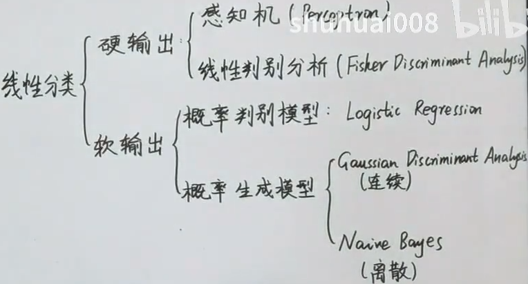
硬输出：0 和 1；或者 +-1

软输出：概率

9 朴素贝叶斯分类器 (Naive Bayes Classifer)

Video-P9

核心思想：朴素贝叶斯假设，又叫条件独立性假设，最简单的概率有向图模型

在给定类别的情况下，属性（维度）之间是相互独立的

随机变量 $y$ 是随机变量，对应 p 维自变量

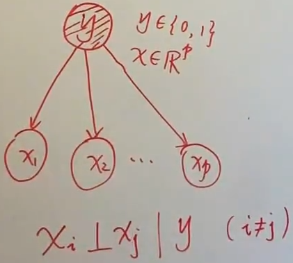
从概率图角度来看，在给定 y 的情况下，从 $x_1$ 到 $x_2$ 的路径被 y 阻断了，所以 $x_1$ 和 $x_2$ 独立。

概率表达式：

假设的动机：为了简化运算， 对于 $\mathbf x = (x_1, x_2, \cdots x_p)^T$，忽略了 $x_i$ 与 $x_j$ 之间的关系，如果p非常大，导致计算困难。

分类数据：$\{(x_i, y_i)\}_{i=1}^N, \ x_i \in \R^p, \ y_i \in {0,1}$，对于一个给定的 x，对它分类：

$$ \begin{aligned} \hat y =& \underset{y}{\operatorname{arg\ max}}\ \underset{后验}{\underline{P{(y|x)}}} \

=& \underset{y}{\operatorname{arg\ max}}\ \frac{P(x,y)}{P(x)}\\

=& \underset{y}{\operatorname{arg\ max}}\ P(y) \cdot P(x|y)

\end{aligned} $$