
Table of contents
(Featured image credits: Least Squares Regression - Math Is Fun Found by Google Lens )
Pseudo Inverse
Source video: 深度学习-啃花书0103伪逆矩阵最小二乘 (2021-07-22) - 科研小灰灰
(2023-02-04)
Solve linear regression
For a n-dimensional linear regression problem,
- There are N input samples: x₁,x₂,…,$x_N$, where each sample is a n-dimension vector xᵢ∈ ℝⁿ
- Their corresponding target outputs are: y₁,y₂,…,$y_N$, where each output is a scalar yᵢ∈ ℝ
Hence, these data can be represented as a linear system:
$$ \begin{cases} x₁₁a₁ + x₁₂a₂ + ... + x₁ₙaₙ = y₁ \\\ x₂₁a₁ + x₂₂a₂ + ... + x₂ₙaₙ = y₁ \\\ \vdots \\\ x_{N1}a₁ + x_{N2}a₂ + ... + x_{Nn}aₙ = y_N \\\ \end{cases} $$Further, this system can be represented with matrix and vector:
$$ \begin{bmatrix} x₁₁ & x₁₂ & … & x₁ₙ \\\ x₂₁ & x₂₂ & … & x₂ₙ \\\ ⋮ & ⋮ & ⋱ & ⋮ \\\ x_{N1} & x_{N2} & … & x_{Nn} \end{bmatrix} \begin{bmatrix} a₁ \\\ a₂ \\\ ⋮ \\\ aₙ \end{bmatrix} = \begin{bmatrix} y₁ \\\ y₂ \\\ ⋮ \\\ y_N \end{bmatrix} $$The objective of the linear regression is to solve the weights vector: $\[ ^{^{a₁}\_{a₂}} \_{^{\ ⁞}\_{aₙ}} \]$ from the linear equation: $𝐗_{N×n} 𝐚_{n×1} = 𝐘_{N×1}$.
If N=n (the coefficient matrix is a square matrix), and the data matrix $𝐗_{N×n}$ is a invertible matrix, then there will be 𝐚=𝐗⁻¹𝐘, such that the weights vector is determined directly.
But in general, the number of samples N is not equal to the number of features n (N ≠ n), that is 𝐗 is not invertible and 𝐚 cannot be represented as 𝐗⁻¹𝐘.
Shift from 𝐗 to 𝐗ᵀ𝐗
Therefore, when the 𝐚 cannot be reached directly, the solution should be as close to the optimal as possible.
That means the objective is to minimize the distance of two vectors:
J=‖𝐗𝐚-𝐘‖² (without constraints)
And the optimal solution is obtained when
∂J/∂𝐚 = 𝐗ᵀ(𝐗𝐚-𝐘) = 0 ⇒ 𝐗ᵀ𝐗𝐚 = 𝐗ᵀ𝐘.
Now, the previous 𝐗 is shifted to here 𝐗ᵀ𝐗 ∈ ℝⁿᕁⁿ, which is a square matrix. And if 𝐗ᵀ𝐗 is invertible, then the optimal 𝐚 can be calculated in one-shot.
Is 𝐗ᵀ𝐗 invertible?
An invertible matrix has to satisfy 2 conditions: it’s a square matrix and its rank equals to the number of variables n (#columns).
According to this video, there are two cases:
-
If N > n, for example N=5, n=3, then (𝐗ᵀ𝐗)₃ₓ₃ is inverible generally. So
𝐚=(𝐗ᵀ𝐗)⁻¹𝐗ᵀ𝐘,
where the coefficient in front of 𝐘, (𝐗ᵀ𝐗)⁻¹𝐗ᵀ, is called the pseudo-inverse matrix. And 𝐚 = (𝐗ᵀ𝐗)⁻¹𝐗ᵀ𝐘 is called the least-square solution. (最小二乘解)
(Because 𝐗 has no inverse matrix, so we find its “pseudo” inverse matrix. Or if 𝐗 is invertible, 𝐗⁻¹=(𝐗ᵀ𝐗)⁻¹𝐗ᵀ, they’re equivalent, but the latter suits more general scenarios.).
-
If $N < n$, for example N=3, n=5, then (𝐗ᵀ𝐗)₅ₓ₅ is not invertible, because:
rank(𝐗ᵀ𝐗) ≤ rank(𝐗₃ₓ₅) ≤ N=3 $<$ n=5.
In this case, 𝐚 cannot be calculated as (𝐗ᵀ𝐗)⁻¹𝐗ᵀ𝐘.
The problem can be understood that there are too many parameters (n is too high). When the parameters are much more than samples, there will be overfitting. And one of the solutions is regularization.
Effect of the regularization term
Since the reason why the optimal solution of the loss function J cannot be solved in one-shot is that there are too many parameters, a regularization is added to the loss funciton as follows:
$$J = ‖𝐗𝐚-𝐘‖² + λ‖𝐚‖², λ>0$$Then the derivative becomes:
∂J/∂𝐚 = 𝐗ᵀ𝐗𝐚 - 𝐗ᵀ𝐘 + λ𝐚 = 0.
By moving items, the equation becomes:
(𝐗ᵀ𝐗 + λ𝐈)𝐚 = 𝐗ᵀ𝐘,
where the (𝐗ᵀ𝐗 + λ𝐈) is invertible. The proof is as follows.
Proof
Since 𝐗ᵀ𝐗 is a symmetric matrix, it can be diagonalized. Thus, 𝐗ᵀ𝐗 can be written as:
$$ 𝐗ᵀ𝐗 = 𝐏⁻¹ \begin{bmatrix} λ₁ & & \\\ & ⋱ & \\\ & & λₙ \end{bmatrix} 𝐏 $$The determinant of 𝐗ᵀ𝐗 is:
|𝐗ᵀ𝐗| = |𝐏⁻¹| ⋅ |$^{^{λ₁}\_{\quad ⋱}} \_{\qquad λₙ}$| ⋅ |𝐏|
= λ₁ ⋅ λ₂ … ⋅ λₙ
And λ₁, λ₂ …, λₙ are the eigen values for the 𝐗ᵀ𝐗
Then the invertibility can be judged from this determinant:
-
If |𝐗ᵀ𝐗| = 0, then 𝐗ᵀ𝐗 is not invertible, because there are some zero lines in the matrix (after elementary row operations), that means rank(𝐗ᵀ𝐗) < n.
-
But if |𝐗ᵀ𝐗| > 0, the matrix 𝐗ᵀ𝐗 is invertible, because it has full rank, which is equal to the number of lines of rows. 【俗说矩阵】行列式等于0意味着什么?你一定要了解哦~ - 晓之车高山老师-bilibili
Analyze the two cases without and with adding the regularization term:
-
Only the 𝐗ᵀ𝐗:
-
Let this matrix be enclosed by a non-zero real row vector 𝛂ᵀ and its column vector 𝛂 to constuct a quadratic form: 𝛂ᵀ(𝐗ᵀ𝐗)𝛂, which is used to characterize the definiteness of 𝐗ᵀ𝐗. Definite matrix -wiki
-
Based on the combination law of the matrix multiplication, it can be written as: (𝛂ᵀ𝐗ᵀ)(𝐗𝛂) = (𝐗𝛂)ᵀ(𝐗𝛂), which is the norm of the vector 𝐗𝛂.
-
Because the norm is ≥ 0 definitely, the 𝛂ᵀ(𝐗ᵀ𝐗)𝛂 ≥ 0 (indicating 𝐗ᵀ𝐗 is positive semi-definite matrix).
-
Based on the properties of quadratic form, eigen values λᵢ of 𝐗ᵀ𝐗 are all ≥ 0
Then the above determinant is |𝐗ᵀ𝐗|= λ₁ ⋅ λ₂ … ⋅ λₙ ≥ 0, so when |𝐗ᵀ𝐗| = 0, the rank of the matrix 𝐗ᵀ𝐗 is not full (≠ n), so the matrix 𝐗ᵀ𝐗 is not invertible.
-
-
For 𝐗ᵀ𝐗+λ𝐈 (where λ is a hyper-parameter), it can be considered as a matrix:
- A quadratic form is constructed as: 𝛂ᵀ(𝐗ᵀ𝐗+λ𝐈)𝛂 = (𝛂ᵀ𝐗ᵀ)(𝐗𝛂) + λ𝛂ᵀ𝛂.
- The second item is always >0 because 𝛂 is not a zero vector, so its norm 𝛂ᵀ𝛂 > 0.
- Therefore, the matrix (𝐗ᵀ𝐗+λ𝐈) is a positive definite matrix. The eigen values λᵢ of (𝐗ᵀ𝐗+λ𝐈) are all > 0.
The determinant of 𝐗ᵀ𝐗+λ𝐈 is the product of its eigen values, i.e., the determinant |𝐗ᵀ𝐗+λ𝐈|>0. So the matrix 𝐗ᵀ𝐗+λ𝐈 has full rank, and 𝐗ᵀ𝐗+λ𝐈 is invertible.
Therefore, the optimal solution can be solved as 𝐚 = (𝐗ᵀ𝐗 + λ𝐈)⁻¹ 𝐗ᵀ𝐘. This is called the “least square - least norm solution”. (最小二乘-最小范数解)
L2 regularization is originally added to make the 𝐗ᵀ𝐗 invertible.
(bilibili search: “伪逆矩阵”)
todo: 01 2、最小二乘与pca(新) - 深度之眼官方账号-bilibili
todo: 【熟肉】线性代数的本质 - 06 - 逆矩阵、列空间与零空间 - 3B1B -bili
todo: 【26 深入理解逆矩阵】- cf98982002 -bili
GPU Solve Inverse
Use GPU to solve inverse faster?
(DDG search: “矩阵求逆 gpu”)
- The acceleration ratio of GPU to CPU is more than 16 times. ⁴.
How to solve inverse matrix?
- Gaussian Eliminate
- LU decomposition, commenly used by computer because it can be performed parallelly.
- SVD decomposition
- QR decomposition
Estimate Polynomial by LS
(2024-06-10)
-
Least-square can be used to approximate the coefficients of a polynomial.
The optimal polynomial corresponds to the minimum error between the observed and predicted values.
Given a point set as below, use a linear polynomial to fit the data:
1
2
x = [0, 0.1, 0.2, 0.3, 0.4, 0.5, 0.6, 0.7, 0.8, 0.9, 1.0] y = [0, 4, 5, 14, 15, 14.5, 14, 12, 10, 5, 4]The general form of a linear polynomial is: ax + b*1 = y, a and b are the coefficients to be estimated:
$$ \begin{bmatrix} 0 & 1 \\\ 0.1 & 1 \\\ 0.2 & 1 \\\ 0.3 & 1 \\\ ⋯ \end{bmatrix} \begin{bmatrix} a \\\ b \end{bmatrix} = \begin{bmatrix} 0 \\\ 4 \\\ 5 \\\ 14 \\\ ⋯ \end{bmatrix} $$$$XA = Y$$-
Obviously, the 2 axes (column space) of X cannot be “recombined” to produce Y space. In other words, the $[^a_b]$ that makes the equation hold doesn’t exist.
Therefore, the objective is shifted to minimize the error between Y_pred and target Y.
-
Project the target Y to the column space of X resulting in Y’ (that will be approximated by A’), and the error: Y’-Y is orthogonal to the column space of X, as the error can’t be explained by the X’s space (Don’t know a theoretical explanation yet).
-
Since Y’-Y is orthogonal to X, there is:
$$\begin{aligned} X^T(Y'-Y)=0 \\\ X^T(XA'-Y) = 0 \end{aligned}$$The best coefficients A’ is:
$$A'=(X^T X)^{-1} X^TY$$
-
-
Use a quadratic polynomial $\rm ax²+bx+c=y$ to fit the data set:
$$ \begin{bmatrix} 0 & 0 & 1 \\\ 0.01 & 0.1 & 1 \\\ 0.04 & 0.2 & 1 \\\ 0.09 & 0.3 & 1 \\\ ⋯ \end{bmatrix} \begin{bmatrix} a \\\ b \\\ c \end{bmatrix} = \begin{bmatrix} 0 \\\ 4 \\\ 5 \\\ 14 \\\ ⋯ \end{bmatrix} $$- x² (e.g., 0.01), x (e.g., 0.1), and 1 are the 3 basis functions that are combined with various ratios to form multiple basiss.
-
On the other hand, the optimal coefficients of a polynomial can also be found by solving the equation that the partial derivative of the error w.r.t. each coefficient equals 0.
Derivation referring to: An As-Short-As-Possible Introduction to the Least Squares, Weighted Least Squares and Moving Least Squares Methods for Scattered Data Approximation and Interpolation (may 2004) - Andy Nealen
Use a quadratic bivariate polynomial to fit a point set (𝐱ᵢ,yᵢ)
$$ \\|Y' - Y\\|^2 $$$$ α = \left[ ∑_{i=1}^N \big( b(xᵢ)⋅ b(xᵢ)^T \big) \right]^{-1} ⋅ ∑_{i=1}^N \big( b(xᵢ) ⋅ yᵢ \big) $$bmeans a basis (a coordinate system), i.e., a series (combination) of basis functions.
Weighted Least Squares
(2024-06-11)
-
The value at each new point is predicted based on an approximated polynomial, which is found by minimizing the difference between the training point and predicted values, and the differences are weighted according to the distance from the new point to each training point.
(2024-06-18)
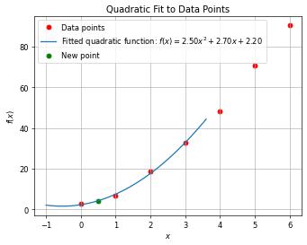
Example: Given 7 points: (0, 2.5), (1, 6.5), (2, 18.5), (3, 32.5), (4, 48), (5, 70.5), (6, 90.5), (data is made up from 2x²+4x+2.5), use WLS to estimate the value at x=0.5.
- LS is featured by its one-shot solution, but I’m not sure what’s the algorithm in
np.polyfit. Just illustrating the general 2 steps below:
-
Approximate a polynomial for only first 4 points:
Code generated by chatGPT4o - Diagrams & Data
Ask: Use a quadratic function to fit the sequence: f(0) =2.5, f(1) = 6.5, f(2) = 18.5, f(3) = 32.5
 1
 2
 3
 4
 5
 6
 7
 8
 9
10
11
12
13
14
15
16
17
18
19
20
21
22
23
24
25
26
27
28
29
30
31
32
33
34
35
import numpy as np import matplotlib.pyplot as plt from numpy.polynomial.polynomial import Polynomial # Given data points x_data = np.array([0, 1, 2, 3]) y_data = np.array([2.5, 6.5, 18.5, 32.5]) # Fit a quadratic polynomial (degree 2) coefs = np.polyfit(x_data, y_data, 2) # Create the polynomial function from the coefficients p = np.poly1d(coefs) # Generate x values for plotting the fitted curve x_fit = np.linspace(-1, 4, 400) y_fit = p(x_fit) # Plot the original data points plt.scatter(x_data, y_data, color='red', label='Data points') # Plot the fitted quadratic function plt.plot(x_fit, y_fit, label=f'Fitted quadratic function:\ $f(x) = {coefs[0]:.2f}x^2 + {coefs[1]:.2f}x + {coefs[2]:.2f}$') plt.title('Quadratic Fit to 4 Neighboring Points') plt.xlabel('$x$') plt.ylabel('$f(x)$') plt.legend() plt.grid(True) # Plot other points plt.scatter(0.5, p(0.5), color='g', label="New point") plt.scatter([4,5,6], [48, 70.5, 90.5], color='r') plt.legend() plt.show() -
Use the estimated polynoimal to infer the value at 0.5:
- LS is featured by its one-shot solution, but I’m not sure what’s the algorithm in
(2024-05-31)
-
Considering some samples (errors) are more important, and the importance is determined by the sample’s neighbors, the loss function becomes: (移动最小二乘法在点云平滑和重采样中的应用-博客园-楷哥)
$$J_{LS} = \sum_{i=1}^N wᵢ (\\^yᵢ - yᵢ)^2$$-
Assume the target function has a “Compact Support”. Thus, each sample is only affected by its neighbors within the local support.
-
Using the variance around a point as the weight.
By only considering a narrow region, each sample has a variance $σᵢ²$. And the weights can be the reciprocal of the variance $\frac{1}{σᵢ²}$:
In other words, WLS takes the correlation of adjacent errors into account. Wikipedia
-
Other reasons analysis: Lecture 24-25: Weighted and Generalized Least Squares - CMU (Found in DDG)
-
-
Examples of fitting circle, line, curves with IRLS: 最小二乘法,加权最小二乘法,迭代重加权最小二乘法 (含代码)【最小二乘线性求解】- CSDN
MLS for Resampling
(2024-06-18)
-
MLS performs WLS repeatedly for all 𝑥 of the function to be approximated, whereas WLS is used to compute the optimal coefficients.
MLS is proposed for fitting surface from discrete data in Surfaces Generated by Moving Least Squares Methods - AMS.
(2024-06-10)
-
The value of a new (querying) point is computed based on its neighboring points in the input (training) point set.
Steps of MLS: (Ref example)
-
Given a point set: (x₁,y₁), (x₂,y₂), (x₃,y₃), …($x_N,y_N$);
-
Predict the value y’ of a new point x’ based on the approximated polynomial, which is found by minimizing the error between the y_pred (evaluated by the approximated polynomial) and the true y values for N points. This minimization process can be performed with a one-shot expression, i.e., pseudo inverse in least squares.
-
The error of each point is scaled by a weight:
$$\sum_{i=1}^N w_i (y_i - y')^2$$where the weight is determined based on the distance from the new point to the training input point:
$$ w = \begin{cases} 0, & \text{dist<0} \\\ \frac{2}{3} - 4 dist^2 + 4 dist^3, & \text{0≤dist≤0.5} \\\ \frac{4}{3} - 4 dist + 4 dist^2 - \frac{4}{3} dist^3, & \text{0.5The optimal coefficients vector 𝛂 of a certain polynoimal is solved based on a “pseudo-inverse form” expression: (Derivation)
$$ α = \big[ ∑_{i=1}^N θ(s) \big( b(xᵢ)⋅ b(xᵢ)^T \big) \big]^{-1} ⋅ ∑_{i=1}^N \big( θ(s) b(xᵢ) ⋅ yᵢ \big) $$sis the distance from the new point to the point i.
-
-
Code demo for resampling with MLS fitting the input point set with a linear polynomial:
 1
 2
 3
 4
 5
 6
 7
 8
 9
10
11
12
13
14
15
16
17
18
19
20
21
22
23
24
25
26
27
28
29
30
31
32
33
34
35
36
37
38
39
40
import numpy as np import matplotlib.pyplot as plt def w(dis): dis = dis / 0.3 if dis < 0: return 0 elif dis <= 0.5: return 2/3 - 4 * dis**2 + 4 * dis**3 elif dis <= 1: return 4/3 - 4 * dis + 4 * dis**2 - 4/3 * dis**3 else: return 0 def mls(x_): sumxx = sumx = sumxf = sumf = sumw = 0 # Iterate every training point to calc coeffs for (a, b) in zip(x, y): weight = w(abs(x_ - a)) # dist2weight sumw += weight sumx += a * weight sumxx += a * a * weight sumf += b * weight sumxf += a * b * weight A = np.array([[sumw, sumx], [sumx, sumxx]]) B = np.array([sumf, sumxf]) ans = np.linalg.solve(A, B) # Calculate y-value at the new point return ans[0] + ans[1] * x_ # Input point set for training: x = [0, 0.1, 0.2, 0.3, 0.4, 0.5, 0.6, 0.7, 0.8, 0.9, 1.0] y = [0, 4, 5, 14, 15, 14.5, 14, 12, 10, 5, 4] # Re-Sampling (for plotting the curve): xx = np.arange(0, 1, 0.01) yy = [mls(xi) for xi in xx] fig, ax = plt.subplots(figsize=(5,5),dpi=50,facecolor="white") ax.plot(xx, yy) ax.scatter(x, y, c='r') plt.show()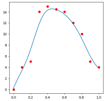
-
MLS smoothing (平滑) means “recomputing” the y-value at each input (training) point x using the found polynomial.
1
2
y_smooth = [mls(xi) for xi in x] ax.scatter(x, y_smooth, c='g')