Code | Arxiv

Notes

Abstract

(2023-05-24)

1. Model the radiance field as a 4D tensor.

   • Optimize a 4D tensor?
   • Optimize a 4D matrix?
   • MLP (network) is a 2D matrix? 𝐗 @ 𝐖ᵀ = 𝐘;
     • Nonlinear regession cannot be solved by linear algebra?
       • Gauss-Newton algorithm

(2023-05-29)

Terminology:

• “4D scene tensor”: (x, y, z, feature). Each voxel is allocated with a sigma and appearance feature. (Alike a feature field?).

  • (2023-10-19) Features on each point derived from the coefficients of each vector in each basis.

• “factorize”: Encode the data into “coordinates” (coefficients) in the principle components;

• “multiple compact”: Principle components are orthogonal between each other;

• “low-rank”: The number of principle components is small. Rank=1 is a vector, rank>1 will depend on the rank of the matrix;

• “component”: The most “iconic sample”, which can be reshaped (reconstructed) to a data that has the original dimensionality,

  • In other words, it’s a “space” constituted by several directions; e.g., an image space has X and Y 2 directions.

  • In TensoRF, a vec + a mat is a component.

  • For a scene placed in a cube, one of components is an equal-sized cube, and the 3 directions are the X,Y,Z axes.

    (2023-10-19) Because the scene is the reconstruction goal, it served as the template of each basis. If the scene isn’t be reconstructed directly, for example, reconstring each ray (ro,rd,l,s), what’s the basis then?

    A 1D signal’s basis is sin+cos.

  • (2023-10-19) Voxels are discrete samples from a continuous scene function. Coefficients on vectors of a basis are inner product between the scene function and each basis. Given some sample points (voxels), their coefficients are the coordinates of their projection onto the basis.

• “mode”: A principle component, a coordinate system, a space, a pattern;

Introduction

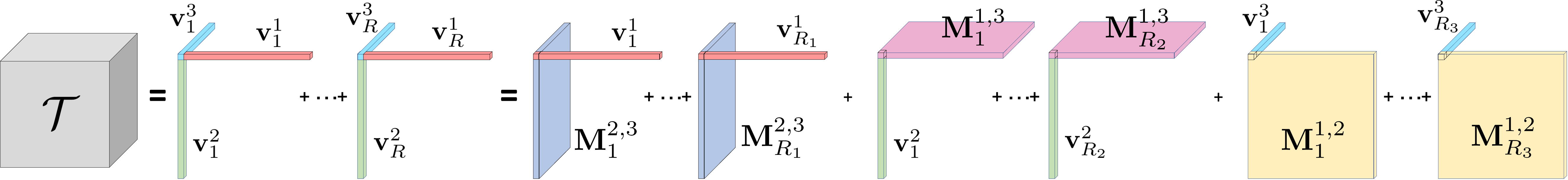
• “CAN-DECOMP/PARA-FAC”: Every direction in a component is a 1-dimensional vector.

• “Vector-matrix decomposition”: two directions out of 3 are jointly represented by a “frame” (plane),

  So the obtained factors for 1 component are 1 vector and 1 matrix.

  

• VM decomposition spends more computation for more expressive components.

  The “similarity” is computed “frame-by-frame”, so it needs more calculation. And the original structure is more kept than 2 dimensions are analyzed individually, so the components could be more representitive and less components are needed.

• Better space complexity: O(n) with CP or O(n²) with VM,

  Comparing with optimizing each voxel directly, which is O(n³), optimizing factors takes less memory.

• Gradient descent

  They’re not encoding the radiance field into factors because the feature grid/tensor is unknown. They decompose the feature grid to simplify the optimization, which then turns to optimizing factors.

Implementation

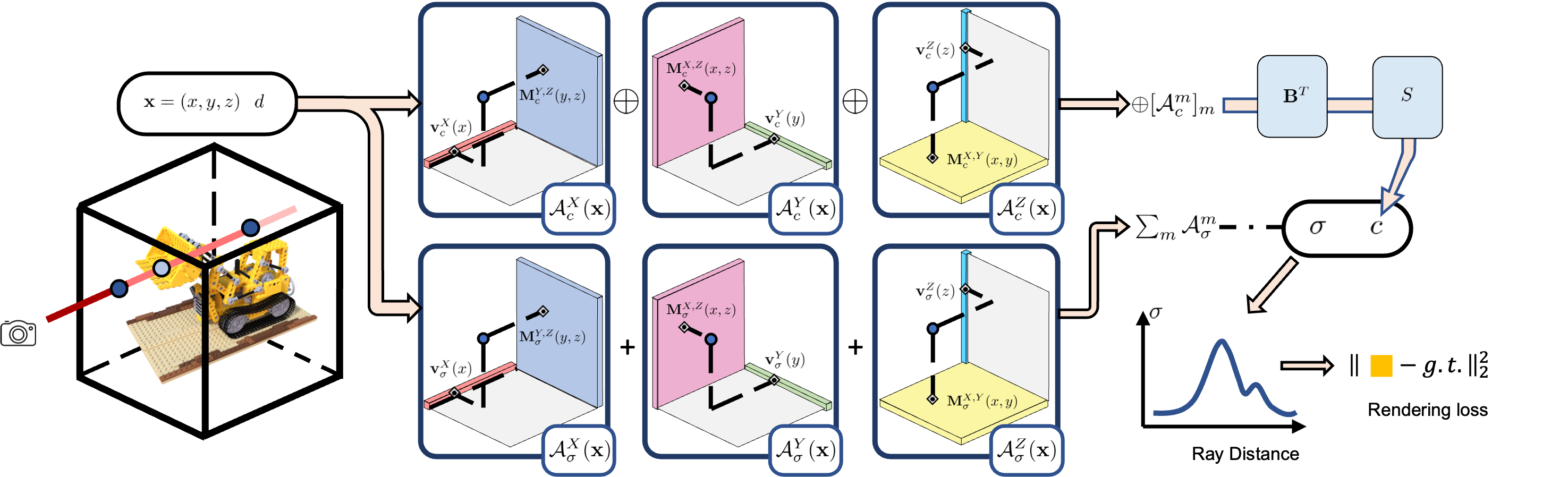
A scene is a radiance field.

Radiance field (4D tensor) = Volume density grid (3D tensor: X,Y,Z) + Appearance feature grid (4D tensor: X,Y,Z,feat)

• Radiance field is a tensor of (X,Y,Z,σ+feature), where volume density σ is 1D, appearance feature is 27D;

• 1D Volume density (feature) is decomposed to 3 vectors (CP) or 3 vector-matrix combo (VM) for each component.

• 27D Appearance feature is amortized into 3 vector-matrix combos for 16 components.

• These components are coefficients to fuse the data “basis vectors” in different ways, which is acting like a network.

• 1D density and 27D features are optimized jointly with coefficients.

  • (2023-10-28) Features and coefficients are optimized simultaneously.

where S is two-layer MLP: 150 → 128 → 128 → 3

• (2023-10-28) I guess the authors came up with tensor decomposition because they realized that Positional Encoding is Fourier decomposition, And NeRF then used MLP to learn the coefficients for the decomposed “Fourier basis”: sin and cos.

Interpolate vector & matrix

Instead of performing tri-linear interpolation at a point by computing 8 corners, a point at arbitrary position is computed by interpolating th vector and matrix.

Code Notes

Steps overview

1. Dataset includes all_rgbs and corresponding ro, and normalized rd under world space all_rays, (N_imgs×H×W, 3)

2. Split the bounding box $[^{[-1.5, -1.5,\ -1.5]}_{[1.5,\quad 1.5,\quad 1.5]}]$ into a voxel grid of the given resolution [128,128,128] determined by the number of voxels args.N_voxel_init

   1	reso_cur = N_to_reso(args.N_voxel_init, aabb)

   Sampling number nSamples = voxel grid diagnoal ∛(128²+128²+128²) / stepSize

Learnable Parameters

init_svd_volume() creates basis vectors and matrices. A vector and a matrix are orthogonal because they’re a side and a plane of a cube.

Parameters to be optimized: 3 Vectors and 3 Matrices

 1
 2
 3
 4
 5
 6
 7
 8
 9
10
11
12
13
14
15
16
17
18
19

def init_one_svd(self, n_component, gridSize, scale, device):
  plane_coef, line_coef = [], []      
  # 3 kinds of vec-mat combo, each combo has 16 components;
  for i in range(len(self.vecMode)): 
    # vecMode: [2, 1, 0]
    vec_id = self.vecMode[i]
    # matMode: [(0,1),(0,2),(1,2)]
    mat_id_0, mat_id_1 = self.matMode[i] 
    
    # (1, 16, 128, 128)
    plane_coef.append(torch.nn.Parameter(
        scale * torch.randn((1, n_component[i], gridSize[mat_id_1], gridSize[mat_id_0]))))

    # (1, 16, 128, 1)
    line_coef.append(torch.nn.Parameter(
        scale * torch.randn((1, n_component[i], gridSize[vec_id], 1))))

  return torch.nn.ParameterList(plane_coef).to(device), 
         torch.nn.ParameterList(line_coef).to(device)

Given a 3D tensor, it can be decomposed as Vector-Matrix combo in three directions:

Each direction has 16 components. In other words, an observation of the cube from a direction can be reconstructed by summing those components up.

doubt: These 3 directions are orthogonal because the cube is viewed from distinct directions, but how are those 16 channels guaranteed to be orthogonal?

• (2023-10-17) Based on the theory of PCA?
• (2023-10-28) Is it possible that 16 components are parallel instead of orthogonal? They’re summed directly, similar to an FC layer with 16 neurons representing 16 ways of combining features.

doubt: Are those components parallel to each other? Do they have different importance or priority?

• (2023-06-22) I guess no. They’re just added together simply.

A scene is decomposed to a set of components, then a scene can be reconstructed using a set of coefficients of those components.

Sepcificlly, each voxel is a summation of the products for corresponding projections on vector and matrix in 3 directions and 16 components.

Based on those vector-matrix components, with the help of interpolation, the value at any location can be obtained.

Filtering rays

Filter the effective rays based on the ratio (deviation) betweem the direction of rays and the direction of bounding box corners.

Mask those rays inside bbox by compareing the ratio of the rd to the direction of the two bbox corners:

 1
 2
 3
 4
 5
 6
 7
 8
 9
10
11
12
13

if bbox_only:
  # Avoid denominator of 0, normalized rd, (chunk, 3)
  vec = torch.where(rays_d == 0, torch.full_like(rays_d, 1e-6), rays_d) 

  # ratio of the direction of bbox corner xyz_min to testing ray
  rate_a = (self.aabb[1] - rays_o) / vec  # (chunk, 3)
  # ratio of the direction of bbox corner xyz_max to testing rd
  rate_b = (self.aabb[0] - rays_o) / vec  

  t_min = torch.minimum(rate_a, rate_b).amax(-1) # [chunk]
  t_max = torch.maximum(rate_a, rate_b).amin(-1) # [chunk]
  # rays located inside the bbox
  mask_inbbox = t_max > t_min

An effective ray should end up inside the bounding box,

✩ is an effective ray, while ◯ is a non-effective ray because it’s out of the bbox.

Reconstruct sigma

The sigma value on each voxel is the summation of 16 components of all 3 directions.

 1
 2
 3
 4
 5
 6
 7
 8
 9
10
11
12
13
14
15
16

# 1D scalar: (args.batch_size*N_samples)
sigma_feature = torch.zeros((xyz_sampled.shape[0],), device=xyz_sampled.device)

# traverse 3 modes
for idx_plane in range(len(self.density_plane)): 

  # interpolate tensor (1,16,128,128) at coordinates (batch_size*N_samples, 1, 2)
  plane_coef_point = F.grid_sample(self.density_plane[idx_plane], coordinate_plane[[idx_plane]],  
      align_corners=True).view(-1, *xyz_sampled.shape[:1]) # (16, batch_size*N_samples)

  # interpolate tensor (1,16,128,1) at coordinates:(bs*N_samples, 1, 2)
  line_coef_point = F.grid_sample(self.density_line[idx_plane], coordinate_line[[idx_plane]],
      align_corners=True).view(-1, *xyz_sampled.shape[:1]) # (16, batch_size*N_samples)

  # accumulate 16 components of 3 directions for each voxel, (batch_size*N_samples)
  sigma_feature = sigma_feature + torch.sum(plane_coef_point * line_coef_point, dim=0)    

The factors grid is composed of 3 planes self.density_plane and 3 vectors self.density_line

The factors corresponding to the sampled 3D points are obtained by F.grid_sample():

Retrieve the “factor in the vector direction” for each sample voxel is like the above figure right.

doubt: Were the coefficients not multiplied with basis vector, but simply summed up together as the reconstruction?

• (2023-06-29) TensoRF is not projecting voxel onto each basis vector (matrix), but retrieving the coefficients from the factor grid.

  What the TensoRF retrieved is the coefficient * vector because it samples the factor grid directly. The factor grid satifies orthogonality naturally, so a coefficient inside is equivalent to having already multiplied with basis vectors.

Reconstruct appear. feature

For appearance feature of each voxel, the vector projection and matrix projection in 3 directions are concatenated together, then multiply together:

 1
 2
 3
 4
 5
 6
 7
 8
 9
10
11
12

plane_coef_point, line_coef_point = [],[]

for idx_plane in range(len(self.app_plane)):
  plane_coef_point.append(F.grid_sample(self.app_plane[idx_plane], coordinate_plane[[idx_plane]],
    align_corners=True).view(-1, *xyz_sampled.shape[:1]))

  line_coef_point.append(F.grid_sample(self.app_line[idx_plane], coordinate_line[[idx_plane]],
    align_corners=True).view(-1, *xyz_sampled.shape[:1]))

plane_coef_point, line_coef_point = torch.cat(plane_coef_point), torch.cat(line_coef_point)

return self.basis_mat((plane_coef_point * line_coef_point).T)

Then RGB is mapped from the appearance featrue:

Optimizing

The learnable parameters includes:

• 16 vectors and 16 matrices for density in 3 directions;
• 48 vec and 48 mat for app feature in 3 directions;
• linear layer transforming 48x3 dim appearance feat to 27D;
• linear layer mapping 27D feat+viewdir to 3-dim rgb.

Losses: L2 rendering loss + L1 norm loss + Total Variation loss.

• TV loss benefits real datasets with few input images, like LLFF.

Q&A

1. How does it ensure that the components are orthogonal during training? (2023-06-10)

Reference

{论文代码阅读}TensoRF: Tensorial Radiance Fields - 爱睡觉的人人