Authors: Yimin Yang; Yaonan Wang; Xiaofang Yuan

Code | TNNLS (2012-06-20)

Try to summary:
(2023-02-15) B-ELM is a variant of I-ELM by dividing the hidden nodes into 2 types: odd and even, which differ in wehther the input parameters (𝐚,b) is randomly generated or calculated by twice inverse operations.

Specifically, the first node is solved from the target 𝐭. Then for subsequent nodes, the even node is solved based on the residual error of its previous odd node.

• The output weights of the odd nodes are calculated as: 𝐇₂ₙ₋₁ʳ + e₂ₙ₋₂ (or 𝐭) ➔ 𝛃₂ₙ₋₁ (➔e₂ₙ₋₁)
• The input weights 𝐚 and bias b of even nodes are solved based on the residual error: e₂ₙ₋₁ ➔ 𝐇₂ₙᵉ ➔ 𝐚,b (➔ ^𝐇₂ₙᵉ ➔ 𝛃₂ₙ ➔ e₂ₙ)
• Note: the superscript r and e stand for “random” and “error” marking the source of H.

Abstract

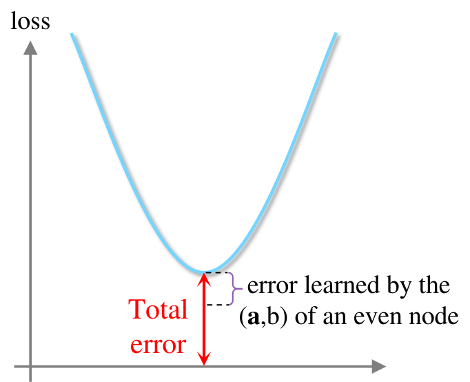
This algorithm tends to reduce network output error to 0

by solving the input weights 𝐚 and bias b based on the network residual error. (In other words, the residual error is represented by a, b of subsequent nodes. Or the error is absorbed by others parameters besides 𝛃.)

Ⅰ. Introduction

For ELM with a fixed structure, the best number of hidden nodes need to ffound by trial-and-error, because the residual error is not always decreasing when there are more hidden nodes in an ELM.

For incremental ELM, the hidden node is added one by one, so the residual error keeps decreasing. But the model training has to do multiple iterations, i.e., calculating inverse matrix is needed after adding each node.

Compared with other incremental ELM, this method is

1. Faster and with fewer hidden nodes
2. showing the relationship between the network output residual error 𝐞 and output weights 𝛃, which is named “error-output weights ellipse”
3. The hidden layer (input weights) with determined parameters instead of random numbers would make the error reduce, or improve the accuracy.

Ⅱ. Preliminaries and Notation

A. Notations and Definitions

⟨u,v⟩ = ∫ₓu(𝐱)v‾(𝐱)d𝐱 is the Frobenius inner product of two matrices u,v, where the overline denotes the complex conjugate.

B. I-ELM

Lemma 1(proved by Huang⁸): indicated that (For the incremental ELM,) the target function can be approximated with more nodes added into the network by reducing the residual error to 0, as the 𝛃 of each new node is calculated based on the error of the network last status eₙ₋₁ as:

𝛃 = $\frac{⟨eₙ₋₁, 𝐇ₙʳ⟩}{‖𝐇ₙʳ‖²}$

The numerator is the inner product measuring the distance from the nth (random) hidden node 𝐇ₙʳ to be added and the error of the network with n-1 hidden nodes.

So the output of the newly added hidden nodes 𝐇ₙʳ are getting smaller and smaller, because they are learning something from the residual error.

Ⅲ. Proposed Bidirectional ELM Method

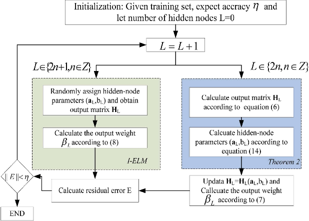
A. Structure of the Proposed Bidirectional ELM Method

Two types of node, the node with odd index {2n-1} has random 𝐚,b, while the 𝐚,b of the node with even index {2n} are calculated based on the residual error of the network with an odd number of nodes at the last moment.

Their output weights both are calculated based on Lemma 1. The 𝐇 of the even node is from residual error, not from the random a,b.

• The odd node aims to approximate the target through 𝐇₂ₙ₋₁ʳβ₂ₙ₋₁, where 𝐇₂ₙ₋₁ is yield based on random a,b;

• The odd node 2n-1 approximates the previous residual error with random generated a,b;

• But the even node approximates the residual error 𝐞₂ₙ₋₁ through 𝐇₂ₙᵉβ₂ₙ with calculated a,b, where 𝐇₂ₙᵉ is yield with the weights a,b solved based on the residual error 𝐞₂ₙ₋₁ from the target (the job hasn’t done by all the previous nodes)

Bi-direction means the approximation is learned from both the target and the error, where the odd node (β₂ₙ₋₁) solved by the target, while the even node (β₂ₙ) calculated by the error. So a pair of odd node and even node is a complete step toward to the target.

Bi-directional means H₂ₙᵉ is calculated first from eq.(6); Then it is calculated again using the ^a,^b, which are solved based on H₂ₙᵉ, to get the updated ^H₂ₙᵉ, which is used to calculate the output weight for the next random odd node based on the Lemma 1.

The dot lines represent the inverse calculation.
β₂ₙ₋₁ is derived from the network residual error of the last status.

Block diagram:

B. Bidirectional ELM method

Theorem 1 states the target function 𝑓 is approximated by the existing network 𝑓₂ₙ₋₂ plus the last two nodes: 𝐇₂ₙ₋₁ʳβ₂ₙ₋₁ and 𝐇₂ₙᵉβ₂ₙ, when n→∞. On the other hand, the residual error the network is 0:

$lim\_{n→∞}‖𝑓-(𝑓₂ₙ₋₂ + 𝐇₂ₙ₋₁ʳβ₂ₙ₋₁ + 𝐇₂ₙᵉβ₂ₙ)‖ = 0$

where the sequence of the 𝐇₂ₙᵉ (the output of the even node calculated from the feedback error) is determined by the inverse of last output weight β₂ₙ₋₁:

$𝐇₂ₙᵉ = e₂ₙ₋₁ ⋅(β₂ₙ₋₁)⁻¹$   (6)

That means $𝐇₂ₙᵉ ⋅ β₂ₙ₋₁ = e₂ₙ₋₁$, this even node is approaching the last residual error based on the known output weight β₂ₙ₋₁.

Then its output weight can be calculated based on the Lemma 1 as:

$β₂ₙ = \frac{⟨e₂ₙ₋₁, 𝐇₂ₙᵉ⟩}{‖𝐇₂ₙᵉ‖²}$   (7)

Once this even node is determined, the corresponding residual error e₂ₙcan be generated, and also the output weight of the next odd node (with 𝐇₂ₙ₊₁ʳ from random weights) can be calculated based on Lemma 1:

$β₂ₙ₊₁ = \frac{⟨e₂ₙ, 𝐇₂ₙ₊₁ʳ⟩}{‖𝐇₂ₙ₊₁ʳ‖²}$   (8)

Theorem 2 further states the updated ^𝐇₂ₙᵉ calculated with the optimal ^a, ^b solved based on 𝐇₂ₙᵉ by the least-square (pseudo inverse) can also let the residual error converge to 0.

Remark 1 clarifies the differences between this method and I-ELM, that is the input weights and bias of even nodes are calculated, not randomly generated. And the output weights are set similarly based on Lemma 1.

Based on the eq. 6, the Δ = ‖e₂ₙ₋₁‖² + ‖e₂ₙ‖² can be reformalized to an ellipse curve.

Code

Training needs to store parameters for each node. And testing needs to query each node sequentially.

Reference

8. G. B. Huang, L. Chen, and C. K. Siew, “Universal approximation using incremental constructive feedforward networks with random hidden nodes,” IEEE Trans. Neural Netw., Jul.2006.