Book site; book

Ⅰ. Curve Fitting

Sec 4.1: Classic Curve Fitting and Least-Squares Regression

Regression ≈ curve fitting ≈ 𝐀𝐱=𝐛 (Least-square fitting), where 𝐀 is the data, 𝐱 is the parameters of the model, 𝐛 is the target.

Regression: Fitting a model to some data with some parameters

Over- and Under-determined

Models could be Over- and Under-determined.

1. Over-determined system normally has No solution.

   There’re massive constraints (equations, samples) given, but the complexity (#variables) of the system is not enough to describe the existing data.

   An over-determined system can be “No solution” or “Infinitely many solution” Over~ wiki

   • Homogeneous case: (no bias)

     • The coefficient matrix is a tall, skinny matrix, the “all-zero solution” always holds.
     • If there’re enough equations are dependent, and after eliminating #non-zero row $<$ #cols in the coefficient matrix in row-echelon form, this over-determined homogeneous system has “infinitely many solutions” (including all-0 solution). Otherwise, “all-zero” is the only solution.

   • Non-homogeneous case:

     • If the last non-zero row of the augmented matrix in row echelon form is only having the constant entry of the last column (giving an equaltion 0=c), this system has “No solution”.

       Since it’s a tall matrix, this case is likely to happen:

       $$ \left[ \begin{array}{cc|c} 2 & 1 & -1 \\ -3 & 1 & -2 \\ -1 & 1 & 1 \\ \end{array} \right] \rightarrow \left[ \begin{array}{cc|c} 2 & 1 & -1 \\ 0 & 5/2 & -7/2 \\ 0 & 3/2 & 1/2 \\ \end{array} \right] \rightarrow \left[ \begin{array}{cc|c} 2 & 1 & -1 \\ 0 & 5/2 & -7/2 \\ 0 & 0 & 13/5 \\ \end{array} \right] $$

       

     • Since the equations are way more than unknowns, the coefficient matrix in row echelon form is most likely not having: #non-zero rows = #cols. So the case “single unique solution” is almost impossible, but there’ll be “Infinite many solutions”.

     • Unless, enough rows can be eliminated (lines overlap), and the remaining coefficient matrix has the same rank as the augmented matrix, and also the #non-zero rows = #cols in the coefficient matrix, this system has “single unique solution”.

   (2024-05-31)

   • 如果约束太多，就变成“超定系统”了，通常无解； 此时就要引入更多的“未知量”，变成一个“欠定系统”，就有无穷多解了

   • 之前我说老弟顾忌的东西太多，无解；所以要引入“变量”。多看多尝试不同的东西，有人就有变数，变则通。

2. Under-determined system normally has infinitely many solutions.

   Because the #parameters is more than equations (samples), some variables are not restricted, which caused the infinitude of solutions. In other words, there’re not enough equations to uniquely determine each unknown. So the problems is how to determine which solution is the best.

   An underdetermined linear system has either No solution or Infinitely many solutions.Under~ wiki

   • Homogeneous case: The coefficient matrix is a short, fat matrix, #non-zero rows $<$ #cols. So the system always has “Infinitely many solutions” (including all-0 solution).
   • Non-homogeneous case:
     • Rank of augmented matrix > Rank of coefficient matrix: No solution
     • Rank of augmented matrix = Rank of coefficient matrix: There must be some solutions. But since the #row is already less than #cols for the coefficient matrix, the single unique solution (except for all-0) is impossible. So this system indeed has infinitely many potential solutions. $$ \left[ \begin{array}{ccc|c} 1 & 1 & 1 & 1 \\ 1 & 1 & 2 & 3 \end{array} \right] \rightarrow \left[ \begin{array}{ccc|c} 1 & 1 & 1 & 1 \\ 0 & 0 & 1 & 2 \end{array} \right] $$

How to solve

1. If there’re infinite optional solutions, then the best model should be selected according to other constraints, i.e., regularizers g(𝐱).

   For instance, the penalty for L2 norm of the parameters vector ‖𝐱‖₂ can lead to the model with smallest mse; And the penalty for L1 norm of the parameters vector ‖𝐱‖₁ can lead to the model with sparse number of parameters.

   Therefore, the objective is:

   $argmin_𝐱 g(𝐱)$ subject to ‖𝐀𝐱-𝐛‖₂=0.

   If some error can be tolerated to just find the model that has the minimum L2-norm params, the constraint can be relaxed by a small error, like: ‖𝐀𝐱-𝐛‖₂≤ε

2. If there’s no solution, the expected model should have the minimum error.

   Therefore, the objective is: $argmin_𝐱$ (‖𝐀𝐱-𝐛‖₂).

   Adding regularizers can confine the optimizer to find the right model, so the objective can be

   $argmin_𝐱$ (‖𝐀𝐱-𝐛‖₂ + λg(𝐱))

   Ordinary least squares gives the approximate solutions (when no exact solution exists) or the exact solution (when it exists) by minimizing the square error:

   $argmin_𝐱$ ‖𝐀𝐱-𝐛‖

   Its solution is 𝐱 = (𝐀ᵀ𝐀)⁻¹𝐀ᵀ𝐛. And using QR factorization of A to solve the least squares can achieve good numerical accuracy.

More broadly, this generic architecture can be generalized to non-linear regressions by replacing ‖𝐀𝐱-𝐛‖₂ to non-linear constraints f(𝐀,𝐱,𝐛):

$$ argmin_𝐱 ( f(𝐀,𝐱,𝐛) + λg(𝐱)) \quad \text{(Over-determined) or} \\ argmin_𝐱 g(𝐱) \ \text{subject to } f(𝐀,𝐱,𝐛) ≤ ε \quad \text{(Under-determined)} $$

An over-determined non-linear system can be solved by Gauss-Newton iteration

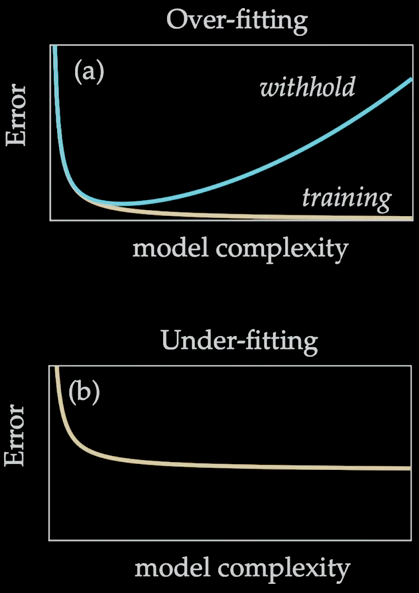
Over- and Under-fitting

Two canonical issues:

1. Over-fitting: With enhencing the model complexity, the training error keeps dropping, but the evaluating error on withhold data goes up.

2. Under-fitting: No matter how you increase the model complexity (parameters), the training error doesn’t drop, either that’s a bad model or there’s not enough data.

Regression framework

Generic Regression: 𝐘 = 𝑓(𝐗,𝛃), input 𝐗 into model 𝑓, then target 𝐘 can be obtained.

Regression needs 2 things: select a model 𝑓 and find its parameters beta that can map X to Y.

Different norms are used to measure the error: L∞ norm, L1 norm, L2 norm. And the selected norm (error metric) has big impact on the “Goodness of Fit”.

Ⅱ. Nonlinear Regression

Sec 4.2: Nonlinear Regression and Gradient Descent

Ⅲ. Regularization

Sec 4.3: Over- and Under-determined Systems; Code demo

Ⅳ. Optimization

Sec 4.4: Optimization for regression

Optimization is the cornerstone of regression.

• Optimization is to minimize some objective function.
• Regression is finding the parameters of the given model that maps the input to the output.

Regularization is Critical

• Regularizers are what determine the type solutions obtained.

Simple Example

The data is generated from parabola + noise $f(x) = x^2 + 𝐍(0,σ)$. However, the model in practice is unknown, and regularization can help find better models.

Given 100 Realizations of data. And the model is represented as $𝐘 = 𝑓(𝐗,β)$

Small noise results complex predicted models.

Different regression

1
2
3

f = (x.^2 + 0.2 * rand(1,n)).';
lambda = 0.1;
phi

1. pinv(): Pseudo-inverse (Least square with the minimum L2 norm)
2. \ (bashslash): QR decomposition
3. lasso()
4. robustfit()
5. ()

Least-square fit pinv get very different model for samll pertubation every time and all the coefficients are functioning. The uncertainty of this solver is high.

The high-dgree terms are highly volatile, which makes the model unstable.

Parsimony (Pareto front) Keep adding higher degree polynomials to the model, the error will no longer decrease at some point and instead even rise up.

Pareto front

Sec 4.7: The Pareto front and Lex Parsimoniae

Small number of parameters can bring interperity

Connect NNs

Sec Neural Networks: 1-Layer Networks