Video 6 Linear Models 9-29-2021

Outline

1. Input representation
2. Linear Classificatin
3. Linear Regression
4. Nonlinear Transformation

Review of Lecture 2

• Learning is feasible in a probabilistic sense.

• Red marble frequence $\nu$ in the bin is unknow → $E_{out}$ is unknown → $E_{in}$: red marble frequence in the sample $\mu$ → 最佳假设 g 使 $E_{in}$ 和 $E_{out}$ 最接近，这时Bad events 的概率为: Ein 和 Eout 相差超过 $\epsilon$ 的概率 $|E_{in}(g) - E_{out}(g)| > \epsilon$

  因为 g 肯定是假设集 H 中 M 个假设的其中之一，每个都有可能:

  $$ |E_{in}(h_2) - E_{out}(h_2)| > \epsilon\ \textbf{ or } |E_{in}(h_2) - E_{out}(h_2)| > \epsilon\ \textbf{ or }\ \cdots |E_{in}(h_M) - E_{out}(h_M)| > \epsilon $$

  也就是 M 个假设对应的Bad events发生概率之和（各假设之间无overlapping，也就是最坏的情况，但通常各假设间有相关性），把M加到Hoeffding Inequality右侧，称为Union Bound：

  $$ P[ |E_{in}(g)-E_{out}(g)|> \epsilon ] \leq 2M e^{-2 \epsilon^2 N} $$

  如果样本数量N足够大，Bad event 的概率就会变小.

Linear model

• Weights are linear related.

• Digits pictures:

  raw input: $\mathbf{x} = (x_0, x_1, \cdots, x_{256})$ (x0是bias)

  linear model: $(w_0, w_1, \cdots, w_{256})$ (inputs constribution,w0=1)

• Features: Extracted useful information （257维太高,线性模型不太行）

  Intensity and symmetry $\mathbf x=(x_0, x_1, x_2)$， $x_0=$bias

  linear model: $(w_0, w_1, w_2)$, $w_0=1$

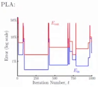
• PLA is not so smart. It focus on one misclassified point and update the weight, then the in-sample error maybe better or worse. There are a lot of flactration during iterations. 错过了最小误差，就回不去了。

  $E_{out}$ 是验证集上的误差，error of out-of-sample follows $E_{in}$

  

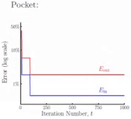
• Pocket: Keep the best weights (in pocket). Replace it when finding better in the future.

  

Linear Classification

• Outputs of a linear model are binary

  $$ h(\mathbf x) = \operatorname{sign} \left( \sum_{i=0}^d w_i x_i \right) : { +1,-1} $$

• +1 or -1 (Approve or Deny)

Linear Regression

• Outputs of a linear model are real-valued

  $$ h(\mathbf x) = \sum_{i=0}^d w_i x_i = \mathbf{w}^T \mathbf{x} \quad \text{(w0 for bias x0)} $$

• 不再传给sign函数，判断$\pm 1$分类

• data set: $\rm (\pmb x_1, y_1), (\pmb x_2, y_2),\cdots (\pmb x_N, y_N)$

  用线性回归去复制 data set，然后预测未来x的y。

• 用假设 $h(\mathbf x) = \mathbf w^T \mathbf x$ 近似未知目标函数 $f(\mathbf x)$:

  $$ \left(h(\mathbf x) - f(\mathbf x) \right)^2 $$

  (Square error will make solving linear regression problem easily one-shot.)

  In-sample error:

  

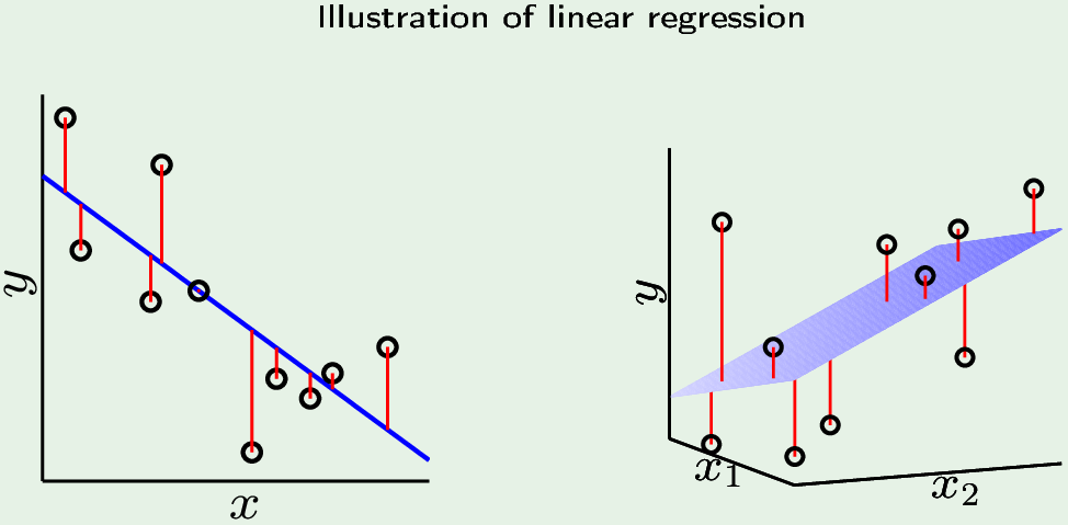
  一个特征是点到直线距离，两个特征是点到超平面距离。

  $$ E_{in}(h) = \frac{1}{N} \sum_{n=1}^N (h(\mathbf x_n) - y_n)^2 $$

  In-sample error 是权重 $\mathbf w$ 的函数 （$\mathbf x$和y都是固定的训练样本,只有$\mathbf w$是变量），线性回归的目标是找到使 In-sample error 最小的$\mathbf w$:

  $$ \begin{aligned} E_{in}(\mathbf w) &= \frac{1}{N} \sum_{n=1}^N (\mathbf w^T \mathbf x_n - y_n)^2 \\ &= \frac{1}{N} | \mathbf{Xw} - \mathbf y |^2 \end{aligned} $$

  （把求和变成矩阵，方便求导找最值）其中：

  $$ \mathbf X= \begin{bmatrix} \mathbf x_1^T \\ \mathbf x_2^T \\ \vdots \\ \mathbf x_N^T \end{bmatrix}, \mathbf y= \begin{bmatrix} y_1^T \\ y_2^T \\ \vdots \\ y_N^T \end{bmatrix} $$

• 求 $E_{in}$ 的最小值：对 $\mathbf w$ 求导，并令其等于0:

  $$ \begin{aligned} E_{in}’(\mathbf w) &= 0 \\ \frac{2}{N} \mathbf X^T (\mathbf {Xw} -y) &= 0 \\ \mathbf X^T \mathbf {Xw} &= \mathbf X^T y \\ \mathbf w &= \mathbf X^{\dagger} y & \text{where } \mathbf X^\dagger = (\bf X^T X)^{-1} X^T \end{aligned} $$

  Perceptron is more similar to the learning process that you’re just trying to learn something from one iteration to the other iteration. Here it’s not iterative. Linear regression is a kind of one-shot learner that learns one iteration.

  $\mathbf X^\dagger$ is the pseudo-inverse of $\mathbf X$:

  $$ \underbrace{ \begin{pmatrix} \underbrace{ \begin{bmatrix} x_{00} & x_{10} & \cdots x_{N0} \ x_{01} & x_{11} & \cdots x_{N1} \ \vdots \ x_{0d} & x_{1d} & \cdots x_{Nd} \end{bmatrix} }_{(d+1)\times N}

  \underbrace{ \begin{bmatrix} x_{00} & x_{01} & \cdots x_{0d} \ x_{10} & x_{11} & \cdots x_{1d} \ \vdots \ x_{N0} & x_{N1} & \cdots x_{Nd} \end{bmatrix} }_{N\times (d+1)}

  \end{pmatrix}^{-1}

  \underbrace{ \begin{bmatrix} x_{00} & x_{10} & \cdots x_{N0} \ x_{01} & x_{11} & \cdots x_{N1} \ \vdots \ x_{0d} & x_{1d} & \cdots x_{Nd} \end{bmatrix} }{(d+1)\times N} }{(d+1)\times N} $$

  $\mathbf w = \mathbf X^\dagger y = \underbrace{[w_0\ w_1\ \cdots w_{d}]}_{(d+1)\times 1}$

Linear regression algorithm

1. 构建 the data matrix $\mathbf X$ and the vector y from the data set $(\mathbf X_1, y_1), \cdots, (\mathbf X_N, y_N)$

   $$ \mathbf X = \begin{bmatrix} \cdots \mathbf x_1^T \cdots \ \cdots \mathbf x_2^T \cdots \ \vdots \ \cdots \mathbf x_N^T \cdots \ \end{bmatrix} , y= \begin{bmatrix} y_1^T \ y_2^T \ \vdots \ y_N^T \end{bmatrix} $$

2. 计算伪逆矩阵 $\mathbf X^\dagger = (\bf X^T X)^{-1} X^T$

3. 返回 $\mathbf w = \mathbf X^\dagger y$

Linear regression for classification

• 利用线性回归一次性解出 $\mathbf w$，将其作为perception的初值，再迭代。
• 1. Linear regression 学习一个实值函数 $y=f(x)$
  2. 二分类函数的 $\pm 1$ 也是实数
  3. 使用linear regression “训练”（学习）到最佳$\mathbf w$（使$E_{in}$(平方误差)最小）$\mathbf w^T \mathbf x_n \approx y_n = \pm 1$
  4. 将这个$\mathbf w$ 作为perceptron的初始值开始训练，随机初始化w可能迭代很多次也不会收敛。

Linear regression boundary

• 线性回归 one-shot 解出的w 对应一条直线.
• 回归是为了使整体的 $E_{in}$ (点到超平面的距离) 最小，当两类数据分布不均匀时，超平面会偏移“分类边界”。in-smaple Error (平方误差)不是Classification error。再用 perception 优化分类结果。

Video 9

Nonlinear transformation

• Use $\Phi$ to transform the non-linear input space $\mathcal X$ to a linear space $\mathcal Z$ (where there is linear relation between $\mathbf w$s)

  Any point $\mathbf x \overset{\Phi}{\rightarrow} \mathbf z$ preserves the linearity, so that points are linearly separable.

• $g(\mathbf x) = \tilde g(\Phi(\mathbf x)) = \rm sign(\tilde \mathbf{w}^T \Phi(\mathbf x))$

• Transformation:

  $$ \begin{aligned} \mathbf x = (x_0, x_1, \cdots, x_d)\ &\overset{\Phi}{\rightarrow} \mathbf z = (z_0, z_1, \cdots, z_{\tilde d}) & \text{维度可以不同,$x_0$是bias} \

  \mathbf{x_1, x_2, \cdots, x_N}\ &\overset{\Phi}{\rightarrow} \mathbf{z_1, z_2, \cdots, z_N} & \text{n个点都做变换}\

  y_1, y_2, \cdots, y_N \ &\overset{\Phi}{\rightarrow} y_1, y_2, \cdots, y_N & \text{标签不变} \

  \text{No weights in } \mathcal X & \qquad \widetilde \mathbf w =(w_0, w_1,\cdots, w_{\tilde d}) & \text{z空间中建立线性模型} \

  g(\mathbf x) &= \rm sign (\tilde \mathbf w^T \Phi(\mathbf x)) \end{aligned} $$