Video 11 Theory of Generalization 10-25-2021
Outline
- Proof that the growth function is polynomial
- Proof that $m_{\mathcal H}(N)$ can replace M
- VC dimension
Examples of polynomial $m_{\mathcal H}(N)$
Proof see the book
Key quantity $B(N,k)$: Maximum number of dichotomies on N points, with break point $k$.
Theorem: $B(N,k) \leq \sum_{i=0}^{k-1} \left( \begin{aligned} N\ i \end{aligned} \right)$
For a given $\mathcal H$, the break point $k$ is fixed:
$$ m_{\mathcal H}(N) \leq \underbrace{ \sum_{i=0}^{k-1} \left( \begin{aligned} N\ i \end{aligned} \right) }_{\text{maximum power is} N^{k-1}} $$
-
Positive ray (break point k=2):
$$ m_{\mathcal H}(N) = C_{N+1}^1 \leq (=) \sum_{i=0}^{k-1} C_N^i = N+1 $$
-
Positive intervals (break point k=3):
$$ m_{\mathcal H}(N) = C_{N+1}^2 + 1 \leq (=) \sum_{i=0}^{k-1} C_{N}^i = \frac{1}{2}N^2 + \frac{1}{2}N + 1 $$
-
2D perceptrons (break point k=4): $$ m_{\mathcal H}(N)=? \leq \sum_{i=0}^{k-1} C_{N}^i = \frac{1}{6}N^3 + \frac{5}{6}N + 1 $$
如果存在 break point, growth function is polynomial function in N : $\sum_{i=0}^{k-1} C_N^i$, whose maximum power is $N^{k-1}$ ($d_{VC}$).
如果没有break point, growth function is $2^N$,就不能保证它是关于N的多项式(最高次幂是 $d_{VC}$,能被e的负幂次抵消),也就不能保证 Bad events 的概率上界足够小,那样就不能通过 Ein 学到Eout。
Proof that $m_{\mathcal H}(N)$ can replace $M$
-
Replace $M$ with $m_{\mathcal H}(N)$ to narrow the upper bound. If M hypotheses are not overlapping, the probability upper bound is very lose.
$$ \begin{aligned} \mathbb P [ |E_{in}(g) - E_{out}(g)| & > \varepsilon] \leq 2\ M\ e^{-2\varepsilon^2 N} \quad \text{(Union bound)} \ & \Downarrow \text{(Not quite)} \ \mathbb P [ |E_{in}(g) - E_{out}(g)| & > \varepsilon] \leq 2\ m_{\mathcal H}(N)\ e^{-2\varepsilon^2 N} \ \end{aligned} $$

长方形中的每个点代表一个样本数据集。 The “flower” represents “bad events” probability (Ein 和 Eout 相差超过$\varepsilon$ 的概率).
Fig (a) 表示的是一个假设的“验证”。While Learning needs to pick the best hypothesis from M hypotheses based on “bad events” probability.
In Fig (b), every hypothesis is not overlapping each other. So their bad events probabilities are taking the whole space, resulting the upper bound maybe very large. 所以不可能通过 $E_{in}$ 学到 $E_{out}$,因为大部分情况下,坏事件发生,它们相差超过了$\varepsilon$。
In Fig (c), many hypotheses overlap together in training data. VC bound 比较小,Ein与Eout 相差超过 $\varepsilon$ 的概率不大。
What to do about $E_{out}$?
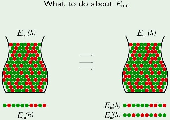
Take another set of samples, called $E_{in}’(h)$. $E_{in}$ 与 $E_{in}’$ 独立同分布,所以 Ein and Ein’ are both following Eout, Ein and Ein’ are following each other.
$$ \begin{aligned} \mathbb P [ |E_{in}(g) - E_{out}(g)| & > \varepsilon] \leq 2\ m_{\mathcal H}(N)\ e^{-2\varepsilon^2 N} \ & \Downarrow \text{(but rather)} \ \mathbb P [ |E_{in}(g) - E_{out}(g)| & > \varepsilon] \leq 4\ m_{\mathcal H}(2N)\ e^{-\frac{1}{8} \varepsilon^2 N} \quad \text{(VC bound)}\ \end{aligned} $$
(Lec7)
The Vapnik-Chervonenkis Inequality:
-
$$ \mathbb P [ |E_{in}(g) - E_{out}(g)| > \varepsilon] \leq 4 m_{\mathcal H} (2N) e^{-\frac{1}{8} \varepsilon^2 N} $$
-
Vapnik-Chervonenkis Inequality 对任何有break point的 hypothesis 都成立。
-
相较于直接用$m_{\mathcal H}(N)$替换M,VC维其实 make the bound worser, larger: $2 m_{\mathcal H}(N) e^{-2\varepsilon^2 N} < 4 m_{\mathcal H} (2N) e^{-\frac{1}{8} \varepsilon^2 N}$
VC dimension
-
VC维 $d_{VC}$ 是某假设集 $\mathcal H$ 最多能完全(二分)分开的点的个数。
$$ d_{VC}(\mathcal H) = k-1 $$
完全分开意味着,假设集$\mathcal H$能分割开由N个点组成的任意的颜色配置:$m_{\mathcal H}(N) = 2^N$
-
有了 $d_{VC}$ 之后:
$N \leq d_{VC}(\mathcal H) \Rightarrow \mathcal H$ can shatter N points
$k \geq d_{VC}(\mathcal H) \Rightarrow k$ is a break point for $\mathcal H$
-
$m_{\mathcal H}(N)$ 的最高维度是 $d_{VC}$
-
Growth function 用 break point k 表示:$m_{\mathcal H}(N) \leq \sum_{i=0}^{k-1} \begin{pmatrix} N \ i \end{pmatrix}$
-
Growth function 用 VC dimension $d_{VC}$ 表示:$m_{\mathcal H}(N) \leq \underbrace{ \sum_{i=0}^{d_{VC}} \begin{pmatrix} N \ i \end{pmatrix} }{\text{minimum power is} N^{d{VC}}}$
-
-
对于不同类型的 hypothesis set:
- $\mathcal H$ is positive rays: $d_{VC}=1$
- $\mathcal H$ is 2D perceptrons: $d_{VC}=3$
- $\mathcal H$ is convex sets: $d_{VC}=\infin$
VC dimension and learning
- 因为 $d_{VC}(\mathcal H)$ 是有限的, 就可以从假设集 $\mathcal H$ 中学习到足够接近未知目标函数 $f$ 的假设g。(保证了Ein与Eout相差很多的概率不大)
- $d_{VC}$ 独立于 learing algorithm, input distribution, target function. 不管它们是什么样,$d_{VC}$只由假设集决定。
VC dimension of perceptrons
- $d_{VC} = d+1$, d is the working dimension of perceptrons (证明见书)
- 例如:2D perceptron 位于 2D plane,所以$d_{VC}=3$; 而 3D perceptron位于3D space,所以$d_{VC}=4$
- $d_{VC} \ (d+1)$ 是权重参数的个数 ($w_0, w_1, \cdots, w_d$)。1 代表bias项,d代表每个样本点的维度数。
Interpreting the VC dimension
-
VC维是自由度 (Degrees of freedom)
不同的weights就是不同的 hypothesis。Every dimension of $d_{VC}$ is a tunable parameter, and parameters create degrees of freedom.
Number of parameters analog degrees of freedom; $d_{VC}$ equivalent “binary” degrees of freedom.
-
The usual suspects
- positive ray: $d_{VC}=1$,一个参数对应一个边界
- positive interval: $d_{VC}=2$,两个参数对应两个边界,确定一个hypothesis
-
Not just parameters
- Parameters 在实际情况中可能不是自由度。
- 每个 perceptron 有 2 个 parameters ($w_0, w_1$ 对应 $b$ 和$x$). So 4 perceptron have 8 parameters those have an impact on a hypothesis, but the $d_{VC}$ maybe not 8.
- $d_{VC}$ measures the effective number of parameters
Number of data points needed
-
经验法则: $N \geq 10 d_{VC}$
-
VC维的两个量化参数: $\varepsilon, \delta$:
$$ \mathbb P [ |E_{in}(g) - E_{out}(g)| > \varepsilon] \leq \underbrace{ 4 m_{\mathcal H} (2N) e^{-\frac{1}{8} \varepsilon^2 N} }_\delta $$
$\delta$是 N 的函数:$N^{d_{VC}} e^{-N}$ ($m_{\mathcal H}(2N)$是N的多项式)
横坐标是 N,纵坐标是概率上界 $\delta$,每条曲线代表不同的VC维:
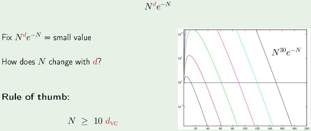
$d_{VC}$越大,概率会先上升得越高,之后负指数take the control,突然急剧减小。因为这是概率,所以只考虑小于1 ($10^0$ 以下)的部分,概率越小越好。
在同一概率下,增加VC维,N的值也呈线性增加。更大的VC维(要调节更多的参数)需要更多的样本点。为了达到很小的 Bad events概率,就需要更多的样本点。
Rule of thumb:(经验) $N \geq 10 d_{VC}$
Rearranging things
-
For VC inequality,把 Bad events 发生的概率称为 $\delta$
$$ \mathbb P [ |E_{out}(g) - E_{in}(g)| > \varepsilon] \leq \underbrace{ 4 m_{\mathcal H} (2N) e^{-\frac{1}{8} \varepsilon^2 N} }_\delta $$
从 $\delta$ 中推出 ε :
$$ \varepsilon = \underbrace{ \sqrt{\frac{8}{N} ln \frac{4 m_{\mathcal H} (2N)}{\delta}} }_\Omega $$
$\Omega$是$N, \mathcal H, \delta$ 的函数。
Good events 表示为:$|E_{out} - E_{in}|\leq \Omega(N,\mathcal H, \delta)$,它的概率是 $P(good) \geq 1-\delta$。
Generalization bound
通常 Eout 比 Ein 大,所以可以去掉绝对值,那么 Good events 就是: $E_{out}-E_{in} \leq \Omega(N,\mathcal H, \delta)$,称为 Generalization error。
然后移项得到 $E_{out}$:
$$ E_{out} \leq \underbrace{ E_{in} + \underbrace{\Omega(N,\mathcal H, \delta)}{\text{Generalization error}} }{\text{Generalization bound}} $$
$E_{in}$ 从训练样本中得知,再根据以上关系,就可得知Eout。