Video 12 Bias-Variance Tradeoff 11-01-2021
Outline:
- Bias and Variance
- Learning Curves
Review of Lec 7
- $d_{VC}(\mathcal H)$: the most number of points $\mathcal H$ can shatter
- $d_{VC}$是有限值,让 g 近似 $f$ 成为可能。VC维仅由假设集决定。
- 为了降低到某一概率,$d_{VC}$越大,所需样本点数N越多。$N\geq 10 d_{VC}$
- $E_{out} \leq E_{in}+\Omega$
- Generalization bound $\Omega(N,\mathcal H, \delta))$:
Bias and Variance
Approximation-generalization tradeoff
近似与泛化的权衡
- 小的Eout 意味着g在 out-of-sample 上也是f的一个好的近似(样本外误差也很小)。
- 越复杂的假设集 $\mathcal H$(M越大),有更好的机会近似 $f$(更可能包含最佳假设g)
- 越简单的假设集 $\mathcal H$,有更好的机会在out-of-sample上泛化。
- 最理想情况:假设集中只包含一个正在寻找的“未知的目标函数” $\mathcal H={f}$,g 也就是f。
Quantifying the tradeoff
- 之前的 VC analysis 是一种评估方法:$E_{out} \leq E_{in}+\Omega$
- 与之相似,Bias-variance analysis 是另一种评估方法:把 Eout 分解成两项:
- 假设集$\mathcal H$ 能有多近似 $f$ (Bias)
- 能在多大程度上确定$\mathcal H$中的好的假设 (Variance)
- 这里分析的目标函数是实值的 real-valued, 并且使用平方误差 squared error
Start with $E_{out}$
Eout 是假设集中的最佳假设 $g$ 与 未知目标函数 $f$ 在输入空间 $\mathcal X$ 的各个点上的差距的期望;g 是样本集 $\mathcal D$ 的函数,样本集不同,选出来的最佳假设 g 也不同:
$$ E_{out}(g^{(D)}) = \mathbb E_{\mathbf x} \left[ \left( g^{(\mathcal D)}(\mathbf x) - f(\mathbf x) \right)^2 \right] $$
因为每次从输入空间抽出的样本集 $\mathcal D$ 不一样,g就不一样,Eout 也就不一样,所以把各个Eout求个期望,作为最终的Eout:
$$ \begin{aligned} \mathbb E_{\mathcal D} \left[ E_{out} \left( g^{(\mathcal D)} \right) \right] = \mathbb E_{\mathcal D} \left[ \mathbb E_{\mathbf x} \left[ \left( g^{(\mathcal D)}(\mathbf x) - f(\mathbf x) \right)^2 \right] \right] \
= \mathbb E_{\mathbf x} \left[ \mathbb E_{\mathcal D} \left[ \left( g^{(\mathcal D)}(\mathbf x) - f(\mathbf x) \right)^2 \right] \right] & \text{(交换位置)} \ \end{aligned} $$
只关注其中 “1个点上的平均误差期望”:$\mathbb E_{\mathcal D} \left[ \left( g^{(\mathcal D)}(\mathbf x) - f(\mathbf x) \right)^2 \right]$
定义平均假设 (average hypothesis):$\bar{g}(\mathbf x) = \mathbb E_{\mathcal D} \left[ g^{(\mathcal D)}(\mathbf x) \right]$ (the best thing you can do),从各不同训练集上得出的最佳假设的平均值。
比如有 K 个训练集:$\mathcal D_1, \mathcal D_2, \cdots, \mathcal D_K$,那么平均假设就是:$\bar{g}(\mathbf x) \approx \frac{1}{K} \sum_{k=1}^K g^{\mathcal D_k}(\mathbf x)$
把平均假设代入"1个点上的平均误差期望":
$$ \begin{aligned} & \mathbb E_{\mathcal D} \left[ \left( g^{(\mathcal D)}(\mathbf x) - f(\mathbf x) \right)^2 \right] \ & = \mathbb E_{\mathcal D} \left[ \left( g^{(\mathcal D)}(\mathbf x) -\bar{g}(\mathbf x) + \bar{g}(\mathbf x) - f(\mathbf x) \right)^2 \right] \quad \text{(减一个加一个)} \
& = \mathbb E_{\mathcal D} \left[ \left( g^{(\mathcal D)}(\mathbf x) - \bar{g}(\mathbf x) \right)^2 + \left( \bar{g}(\mathbf x) - f(\mathbf x) \right)^2 + 2 \left( g^{(D)}(\mathbf x)-\bar{g}(\mathbf x) \right) \left( \bar{g}(\mathbf x) -f(\mathbf x) \right) \right] \quad \text{(代入括号)} \
& = \mathbb E_{\mathcal D} \left[ \left( g^{(\mathcal D)}(\mathbf x) - \bar{g}(\mathbf x) \right)^2 \right] + \underbrace{\mathbb E_{\mathcal D} \left[ \left( \bar{g}(\mathbf x) - f(\mathbf x) \right)^2 \right]}{与D无关,期望还是自己} + 2 \left( \underbrace{ \mathbb E{\mathcal D} \left[ g^{(D)}(\mathbf x) \right] -\bar{g}(\mathbf x) }_{相等, =0} \right) \left( \bar{g}(\mathbf x) - f(\mathbf x) \right) \
& = \underbrace{ \mathbb E_{\mathcal D} \left[ \left( g^{(\mathcal D)}(\mathbf x) - \bar{g}(\mathbf x) \right)^2 \right] }{\rm var(\mathbf x)} + \underbrace{ \left( \bar{g}(\mathbf x) - f(\mathbf x) \right)^2 }{\rm bias(\mathbf x)} \end{aligned} $$
$\bar{g}(\mathbf x)$ 是"最佳假设",它与目标未知函数的差是常数 bias (与D无关),而 $g^{\mathcal D}(\mathbf x)$ 随训练集不同,会上下波动,与"平均值"的差的平方,再取平均就是方差。 各个最佳假设与目标未知函数的平方误差的期望,被拆成了两部分:各最佳假设与平均假设的方差,加上平均假设与目标未知函数的平方误差。
所以 Eout 等于:
$$ \begin{aligned} & \mathbb E_{\mathcal D} \left[ E_{out} (g^{(\mathcal D)}) \right] \ & = \mathbb E_{\mathbf x} \left[ \mathbb E_{\mathcal D} \left[ \left( g^{(\mathcal D)}(\mathbf x) - f(\mathbf x) \right)^2 \right] \right] \ & = \mathbb E_{\mathbf x} \left[ \rm bias(\mathbf x) + var(\mathbf x) \right] \ & = \rm bias + var \end{aligned} $$
The trade off between bias and var
bias = $\mathbb E_{\mathbf x} \left[ \left( \bar{g}(\mathbf x) - f(\mathbf x) \right)^2 \right]$
variance = $\mathbb E_{\mathbf x} \left[ \mathbb E_{\mathcal D} \left[ \left( g^{(\mathcal D)}(\mathbf x) - \bar{g}(\mathbf x) \right)^2 \right] \right]$
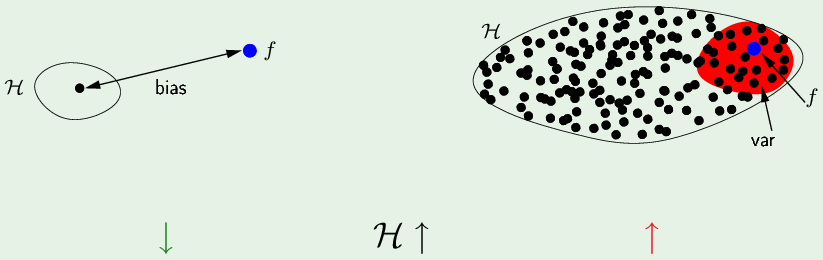
如果假设集中只有一个假设 h,它与 $f$ 的距离就是 bias(方差为0)。如果是一个复杂的假设集,其中包含很多假设,更有可能囊括了 f,在它附近的都是“最佳假设”(红色),因为平均假设$\bar g(\mathbf x)$就在 f 附近所以bias较小,而方差比较大(很多小值加起来也会大)。
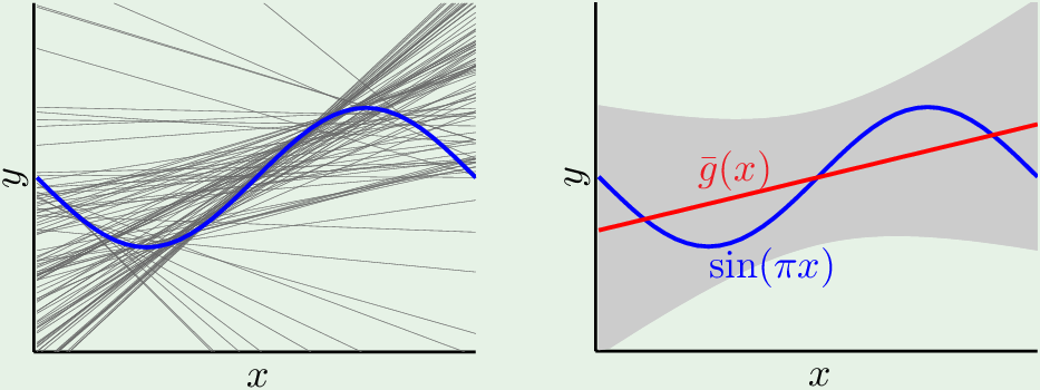
Example: sine target
近似正弦曲线,未知目标函数 $f(x) = sin(\pi x)$,把 f 从输入空间从 [-1,1] 扩展到实数域 $f:[-1,1] \rightarrow \mathbb R$。只有两个样本点 N=2。
有两个假设集,自由度不同:
$$ \begin{aligned} & \mathcal H_0 : h(x) = b &{\text{各假设只有一个参数b (常数)}} \ & \mathcal H_1 : h(x) = ax+b &{\text{各假设有两个参数a,b (直线)}} \end{aligned} $$
Approximation: 上帝视角可以看出两个假设集中的最佳假设(bias最小)分别应该为:
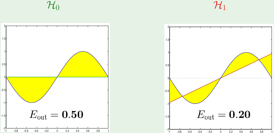
黄色区域是 bias (或者说就是 Eout, 因为单个假设的方差为0)。所以在近似[-1,1]区间上的正弦函数时,$\mathcal H_1$ 比 $\mathcal H_0$ 的 bias 更小。
Learning: 两个样本点的位置是随机的
如果一开始两个样本点位置如图:
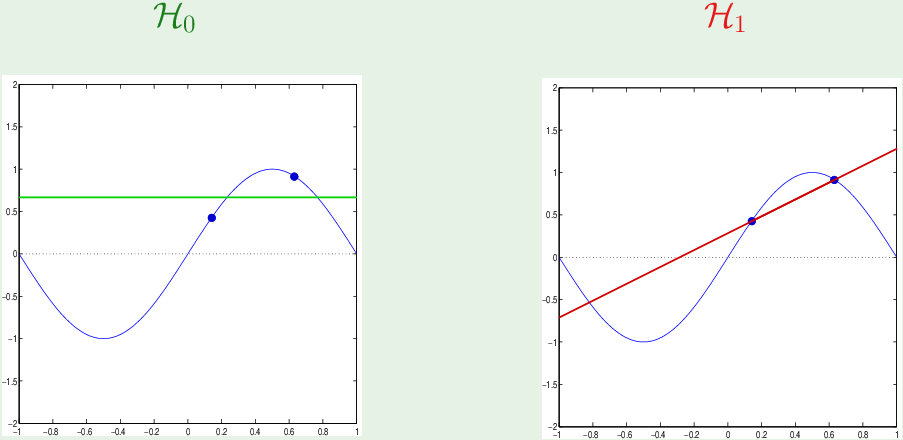
为了使 bias 最小,$\mathcal H_0$中的“最佳假设”应该在两样本点中间,$\mathcal H_1$ 中的“最佳假设”应该穿过两个样本点。
两个样本点(训练集)每次从输入空间中取的都不一样,对应的“最佳假设”也有很多种可能:
对于假设集 $\mathcal H_0$,最佳假设的分布如图:
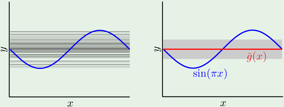
对各个“最佳假设”取平均,平均假设位于”平衡位置“,灰色区域是 variation.
对于假设集 $\mathcal H_1$,最佳假设(过两样本点的直线)的分布如图:
平均假设是红色直线,灰色区域是variation。
对比两个假设集:
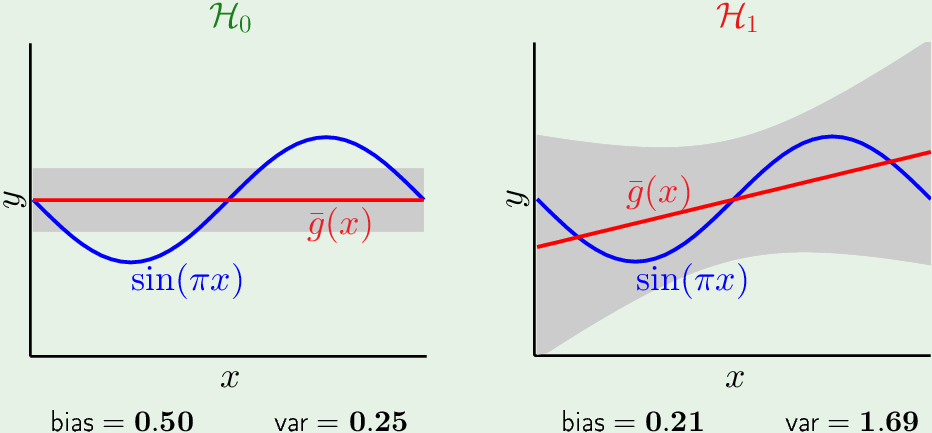
只有一个参数的,最简单的(常数)假设集 $\mathcal H_0$ 的(平均假设) bias大,方差小。而比较复杂的(直线)假设集 $\mathcal H_1$ 的 bias 小,方差大。
最终,$\mathcal H_0$ 的 Eout= 0.50+0.25 = 0.75,$\mathcal H_1$ 的 Eout=0.21+1.69 = 1.9。根据 Eout,简单的假设集 $\mathcal H_0$ 好于复杂的假设集 $\mathcal H_1$。因为我们是从 Ein “泛化” 到 out,如果Eout 太大,Generalization bound 太大,Ein 与 Eout 相差太大,二者不follow,就不能通过Ein 学习到 Eout.
复杂的(自由度多的)假设集有很好近似能力,但是学习能力很差,因为方差太大,不一定能学到最佳假设。
Lesson learned: 模型的复杂度应该匹配 数据(样本决定了最终找出的假设),而不应该匹配目标函数的复杂度。比如只有15个样本,假设已知目标函数是10阶的。你可以选1阶,2阶的模型,它们对应的参数有2个,3个,按照经验法则 $N>10 d_{VC}$,它们至少需要20个,30个样本。但现在只有15个,如果你觉得1阶(直线)不太可能的话,可以用2阶(二次函数)。如果用10阶模型,就出现过拟合了。
Learning Curves
Ein 与 Eout 的曲线。
对于任意有N个(训练)样本数据集 $\mathcal D$。
Expected Eout = $\mathbb E_{\mathcal D} \left[ E_{out} \left( g^{(\mathcal D)} \right) \right]$ (不同测试集上的最佳假设 g 的平均)
Expected Ein = $\mathbb E_{\mathcal D} \left[ E_{in} \left( g^{(\mathcal D)} \right) \right]$ (不同(训练)数据集上的最佳假设 g 的平均)
它们随 N 如何变化?(How do they vary with N?)
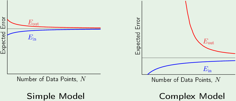
对于Simple Model(的假设集),随着样本数不断增加,Eout越来越小,越来越近似 f,而 Ein越来越大,因为每个样本都有误差,样本越多加起来越大。N越大,Ein与Eout越接近,Generalized bound越小,收敛于 “平均假设” (黑色水平线)。
对于Complex Model,“平均假设”更靠近 f,bias较小,所以黑色水平线它更低,同样随着N增大,Eout与Ein 不断趋近于 “平均假设”。但是当N很小的时候,Eout很大(方差很大)。Eout 与Ein 差距很大,复杂模型相较于简单模型的 Generalization bound 更大。复杂模型的 Ein 在样本很少的时候是零,因为在样本数小于VC维或者假设集的effective参数自由度时,模型可以把所有点全部分开 (shatter all the points)。在超过VC维之后,Ein开始增加。
VC vs Bias-variance
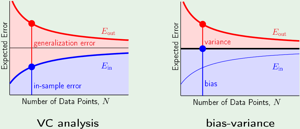
在 VC 分析中,$E_{out} = E_{in} + \text{Generalization error}$
在 Bias-variance 中,不再关注$E_{in}$,因为 $E_{out}=\text{var + bias} = \mathbb E_{\mathcal D} \left[ \left( g^{(\mathcal D)}(\mathbf x) - \bar{g}(\mathbf x) \right)^2 \right] +\mathbb E_{\mathcal D} \left[ \left( \bar{g}(\mathbf x) - f(\mathbf x) \right)^2 \right]$,Eout 等于“粗黑线”(average hypothesis, bias)加上variance。bias取决与假设集而与N无关,所以bias是直线。
随着N增大,它们都趋近于平均假设。所以都需要tradeoff:简单的模型近似能力差,但它 Generalization error小;复杂的模型近似能力强,但它需要更多的样本,才能减小 Generalization bound。对于复杂的模型,样本数越少,Eout越大。样本少的时候,简单模型的Eout 可能比复杂模型的 Eout 还要小。所以样本少选简单模型,样本多选复杂模型。
Linear Regression case
Noisy target $y = \mathbf w^{*T} \mathbf x$ + noise (用线性模型, 从有噪声的样本中,学习一个线性目标函数)
Data set $\mathcal D = { (\mathbf x_1, y_1), \cdots, (\mathbf x_N, y_N) }$
Linear regression solution: $\mathbf w = (\mathbf X^T \mathbf X)^{-1} \mathbf X^T \mathbf y$
In-sample error vector = $\bf X w - y$
“Out-of-sample” error vector = $\bf X w - y’$ (使用相同的x, noise不同,得到测试集)
有了上面非常特殊的情况,才能得到下面的公式:
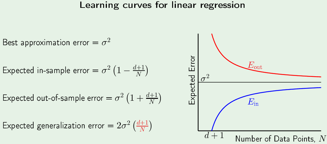
$\sigma^2$ 是 energy of the noise。一个 zero-mean noise的energy 与variance 成正比,