Normalize Dataset

(2023-11-23)

Normalizing a dataset means making the variance to 1.

方差是一个标量（偏离期望的平方的期望）: the average of squared difference between each value in a dataset from the mean value.

• Square ignores the sign of deviations, and only focuses on magnitudes.

• Given 2 datasets with different scales: 1,2,6 and 10,20,60.

  1 2	-*--*--▲------* V.S. -*--*--▲------* 1 2 3 6 10 20 30 60

  Their variance are 4.66 and 46.6. After normalization, their variance will both become 1. (Plain number, without any practical meaning.)

• Transform the variance to 1: subtract mean and divide by std for each sample.

  $$ Var = \frac{∑(\frac{x-μ}{σ} - 0)²}{n} = \frac{∑\frac{(x-μ)²}{σ²}}{n} = \frac{1}{σ²} σ² = 1 $$

• The consequences of normalization have 2 aspects:

  1. Because all the squared deviations (x-μ)² are scaled by their average: σ², the measuring unit is eliminated (消除量纲). Hence, different attributes (dimensions) can be compared equally.

  2. On the other hand, the sum of the scaled squared deviation becomes $n$. Thus, the new variance is 1.

     $$ Var = \frac{∑\frac{(x-μ)²}{σ²}}{n} = \frac{∑\frac{(x-μ)²}{ \frac{∑(x-μ)²}{n} }}{n} = \frac{n ∑\frac{(x-μ)²}{∑(x-μ)²} }{n} = \frac{n* 1}{n} =1 $$

     • Analogy: $\frac{a}{a+b+c} + \frac{b}{a+b+c} + \frac{c}{a+b+c}=1$

• Variance can be scaled to any value. Taking 1 is for interpretability and simplifying calculations (?)

(2023-01-14)

BatchNorm

BatchNorm: 前向过程中每层的输入的分布一直在变化，不满足独立同分布，导致内部协变量偏移Internal Covariate Shift问题， 所以对每层的激活值在输入下一层之前，把这一个batch的分布调整为0均值，方差为1的标准正态分布， 即固定每个隐层节点的激活输入分布，让输入的激活值落在激活函数梯度较大的区域，加快收敛与避免梯度消失。 Batch Normalization导读-张俊林-知乎

• (2024-02-21) 不是“正态分布”，标准化不会改变数据的分布类型，数据原来是什么分布，做完 normalization 还是什么分布。 (mean=0, sigma=1) 只是一个 标准，之后经过一些运算，分布的参数发生变化了，还可以回到这个标准。

todo: L11.2 How BatchNorm Works

todo: L11.4 Why BatchNorm Works

Normalization layer 对数据减均值，除以标准差。以下的 N 是一个 batch 中的样本个数(batch size, B)， 图片batch：(N,C,H,W)，序列batch: (N, embed_dim, seq_len)。 1d,2d,3d方法的区别在于 input 的维度。 Learnable parameters 是γ 和 β 用于对 μ和σ 做 affine 变换。 running mean 和 running var 在训练时不断使用在前向时得到的 x 的mean 和 var 做加权更新，权重为动量 momentum

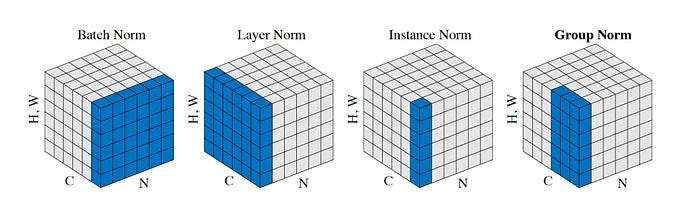
• BatchNorm 让1个batch的，每个通道的均值为0，方差为1（整个batch的μ也=0）；
  指定通道数量input.shape[1]: bn=nn.BatchNorm1d(num_features=C)

• LayerNorm 让每个样本的全部通道（最后几维，一个单词的特征向量，一幅图片的feature map）的均值为0，方差为1，layer指的是 fc net 的一层；
  指定最后几维: ln=nn.LayerNorm(normalized_shape=[C,H,W])）

• InstanceNorm 让每个样本的每个通道的均值为0，方差为1，同一batch内的样本没有联系，用于风格迁移；
  指定通道数量: in=nn.InstanceNorm1d(num_features=C)

• GroupNorm 介于 LayerNorm 和 Instance Norm之间，通道分组=1 就是LN，通道分组=C 就是IN；
  指定通道分组: gn=nn.GroupNorm(num_groups=2, num_channels=C) lecture 7b 神经网络的训练(归一化，迁移学习）-ranchlai-bili; github repo

  Wu&He ECCV2018

• Weight Norm

(2023-08-03)

LayerNorm Customize

• LayerNorm, as referring to ConvNeXt-meta’s nn.LayerNorm, can only normalized the last few channels.

• F.layer_norm can be used to normlize one of the middle dimensions, as in ConvNeXt-torchvision

Loop of ChatGPT’s Wrong Solutions:

1. Q: In the following code, why is the grad of self.weight None after loss.backward()?

   1 2 3 4 5 6 7 8 9 10 11 12 13 14 15 16 17 18 19 20 21 22 23 24 25 26 27 28 29 30 31 32 33 34 35

   class LayerNorm(nn.Module): r""" Input data: (batch_size, C, H, W) Use F.layer_norm to do normalization for the dim of channels. """ def __init__(self, eps=1e-6): super().__init__() self.normalized_shape = (4, ) # C = 3, placeholder self.weight = nn.Parameter(torch.ones(self.normalized_shape)) self.bias = nn.Parameter(torch.zeros(self.normalized_shape)) self.eps = eps def forward(self, x): r""" Since the `normalized_shape` (#channels) of x is unknown when initializing the model, implement normalization for the channels dimension here. """ if self.normalized_shape != (x.shape[1],): self.weight = nn.Parameter(torch.ones(x.shape[1])) self.bias = nn.Parameter(torch.zeros(x.shape[1])) mean = torch.mean(x, dim=1, keepdim=True) var = torch.var(x, dim=1, correction=0, keepdim=True) # biased estimation x = (x - mean) / torch.sqrt(var + self.eps) x = self.weight[:, None, None] * x + self.bias[:, None, None] print(x.shape) return x x = torch.ones(1,3,224,224) myLN = LayerNorm() myLN.weight.register_hook(lambda grad: print(grad.shape)) normalized_x = myLN(x) target_x = torch.rand(1,3,224,224) loss = nn.MSELoss()(normalized_x, target_x) loss.backward()

   Answer:

   The redefined variables self.weight, self.bias inside the forward method are not part of the computation graph, so their gradients won’t be computed during the backward pass.

   And the new created parameter tensors have no connection to the original self.weight and self.bias (created during initialization), which are not used in the forward pass. so their grad attribute remain None.

   Finally, he suggested me don’t redefine in the forward.

2. Q: But I don’t have information about the shape of self.weight to initialize it inside the init method.

   Answer:

   Initialize them as None in the __init__ method and then initialize them with the correct shape during the first forward pass.

   1 2 3 4 5 6 7 8 9 10 11 12 13 14 15 16 17 18 19 20 21

   class LayerNorm(nn.Module): def __init__(self, eps=1e-6): super().__init__() self.eps = eps self.normalized_shape = None # Placeholder for the shape of self.weight self.weight = None # Placeholder for the weight parameter self.bias = None # Placeholder for the bias parameter def forward(self, x): if self.normalized_shape is None: # Initialize self.normalized_shape and create weight and bias with the correct shape self.normalized_shape = (x.shape[1],) self.weight = nn.Parameter(torch.ones(self.normalized_shape)) self.bias = nn.Parameter(torch.zeros(self.normalized_shape)) print(self.bias.shape) mean = torch.mean(x, dim=(2, 3), keepdim=True) var = torch.var(x, dim=(2, 3), correction=0, keepdim=True) x = (x - mean) / torch.sqrt(var + self.eps) x = self.weight[:, None, None] * x + self.bias[:, None, None] print(x.shape) return x

3. This code has an ValueError: optimizer got an empty parameter list

   Anwser:

   Apologies for the oversight. The error is happening because the LayerNorm class does not define any learnable parameters (weights and biases) in its __init__ method. As a result, when you try to pass myLN.parameters() to the optimizer, it doesn’t find any parameters to optimize, leading to the “optimizer got an empty parameter list” error.

   In order to use an optimizer like Adam, you need to define at least one learnable parameter within your model that will be optimized during training.

   Since you don’t have information about the shape of the input during initialization, you can create a placeholder for self.weight and self.bias in the __init__ method, and then initialize them with the correct shape during the first forward pass. To do this, we can use the register_buffer method, which allows us to create tensors that are not optimized during training but still part of the model.

   Here’s the updated code with the use of register_buffer:

   1 2 3 4 5 6 7 8 9 10 11 12 13 14 15 16 17 18 19 20 21 22

   class LayerNorm(nn.Module): def __init__(self, eps=1e-6): super().__init__() self.eps = eps self.register_buffer('normalized_shape', torch.tensor([])) self.register_buffer('weight', torch.tensor([])) self.register_buffer('bias', torch.tensor([])) def forward(self, x): if self.normalized_shape.numel() == 0: # Initialize self.normalized_shape and create weight and bias with the correct shape self.normalized_shape = torch.tensor([x.shape[1]]) self.weight = nn.Parameter(torch.ones(self.normalized_shape)) self.bias = nn.Parameter(torch.zeros(self.normalized_shape)) print(self.bias.shape) mean = torch.mean(x, dim=(2, 3), keepdim=True) var = torch.var(x, dim=(2, 3), correction=0, keepdim=True) x = (x - mean) / torch.sqrt(var + self.eps) x = self.weight[:, None, None] * x + self.bias[:, None, None] print(x.shape) return x

   Now the model will contain learnable parameters that can be optimized using an optimizer like Adam. The grad attribute of self.weight should be available and updated after loss.backward().

   Additionally, you can also use torch.nn.init functions to initialize the weight and bias tensors in a more standard way. For example, you can use torch.nn.init.ones_ and torch.nn.init.zeros_ to initialize the self.weight and self.bias tensors, respectively.

4. register_buffer doesn’t add parameters to optimizer to optimize neither.

It may be necessary to know the number of channels.

• Just sum up the attribute out_chnnels of each layer, e.g., alexnet.features[0].out_channels. PyTorch Forum

  But Swin transformer doesn’t have Conv2d.

• Maybe I can only hard code the numbers of channels.

• If you add the norm layer following the convolution layer, the normalized_shape is the out_channels of the convolution layer.

  But here, I want to normalize the stacked extracted feature maps. So I need to know the total channels of the incoming feature maps.

If the #channels is known, I can use F.layer_norm() directly.

(2023-10-17)

Absorb BN

1. Normalization is performed to keep each “stage” (layer) in a network maintain the same distribution, such that the training could be more efficient due to

   1. Leaving out modeling distributions shift of each layer’s input data.

   2. Stabilizing optimization by suppressing “outliers” (high value) in the output feature map of each layer to avoid big variations in the final prediction.

      Refer to: BN、BN同步、吸收BN - EveK的文章 - 知乎

2. Specifically, input data has (mean=0, std=1), but after a conv layer, the outcome feature maps may don’t persist (mean=0, std=1).

   1. Ideally, featue maps’s distribution should be transformed to (mean=0, std=1) to align with the input data. And that transformation requires its whitening matrix , which transforms co-variance matrix of the feature maps an identity matrix, meaning each dimension is unrelated. CSDN

      However, solving the whitening matrix for a high-dimension tensor is time consuming.

      Therefore, the “whitening” is performed only for each channel.

   2. On the other hand, it’s difficult to get the exact distributions at once, because the data is trained batch-by-batch.

      Therefore, the distribution to be corrected pertains only to the small batch of data. (Or involving previous data by using moving average of history mean and std)

      And only 2 parameters (mean, std) of their distribution are considered to keep the distributions consistent.

3. Once a feature map $M_{(N, C, H, W)}$ spit out from a conv layer, BatchNorm normalizes the data at the same channel for all N samples in the batch:

   \begin{algorithm}
   \begin{algorithmic}
   \FOR {i=0 \TO M.size(1)}
     \PROCEDURE{BN}{ M, meanʰ, stdʰ, scale, bias}
       \STATE mean = M[:, i, :, :].sum() / N   
   
       \STATE std = ( (M[:, i, :, :] - mean)² / N ).sqrt()
   
       \STATE M⁰¹ = (M[:, i, :, :] - mean) / std
   
       \STATE M' = scale * M⁰¹ + bias
     \ENDPROCEDURE
   \ENDFOR
   \end{algorithmic}
   \end{algorithm}
   

   • meanʰ and stdʰ are from history.

   • The scale factor γ and bias β are for the situation where the variation is very small. Then the differences can be magnified through scaling to avoid representation capacity degradation.

   • And γ,β are required to be learnable to automatically find the appropriate feature levels. Otherwise, bias will grow to infinity as explained in paper.

4. Combine BN into wights and bias of the last layer

   $$ M’ = γ \frac{M - mean}{std} + β = \frac{γ⋅M}{std} \left( β - \frac{γ ⋅ mean}{std} \right) $$

   If M is calculated as $M = w⋅x + b$, by substituting it, the equation becomes:

   $$ M’= \frac{γ⋅w}{std} x + \left( β - \frac{γ⋅mean}{std} + \frac{γ⋅b}{std} \right) $$

   Thus, w becomes $\frac{γ⋅w}{std}$ and b becomes $( β - \frac{γ⋅mean}{std} + \frac{γ⋅b}{std} )$.

5. Given a conv layer with $C_i$ input channels and $C_o$ output channels, BN for this layer has $C_i × C_o$ parameters, where $C_i$ is for the history channels, $C_o$ is for target channels.