Jacobian matrix
Prerequisite
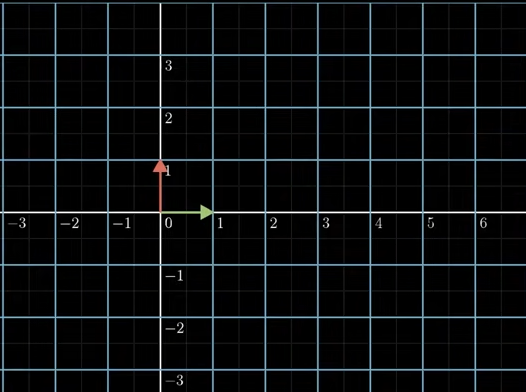
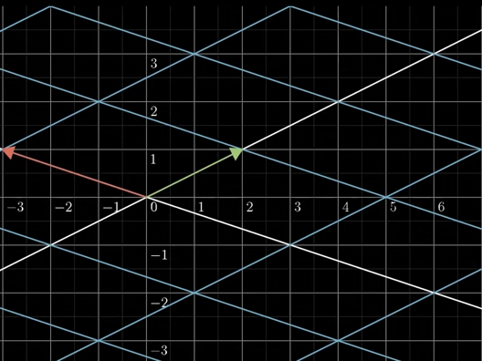
Matrix is a linear transformation of space by moving the basis vectors to new landing spot.
$$ \begin{bmatrix} 2 & -3 \\ 1 & 1 \end{bmatrix} \begin{bmatrix} x \\ y \end{bmatrix} \rightarrow \begin{bmatrix} 2x + (-3)y \\ 1x+1y \end{bmatrix} $$

|

|
-
“linear”: grid lines remain parallel, evenly spaced and straight lines after transformation.
-
Transform
The two basis vectors $[^1_0]$ and $[^0_1]$ are moved to $[^2_1]$ and $[^{-3}_{1}]$, which are the columns of the matrix.
$$ \begin{array}{ccc} \begin{bmatrix} 2 & -3 \\ 1 & 1 \end{bmatrix} \begin{bmatrix} 1 \\ 0 \end{bmatrix} = \begin{bmatrix} 2+0 \\ 1+0 \end{bmatrix} \\ \\ \begin{bmatrix} 2 & -3 \\ 1 & 1 \end{bmatrix} \begin{bmatrix} 0 \\ 1 \end{bmatrix} = \begin{bmatrix} 0-3 \\ 0+1 \end{bmatrix} \end{array} $$
-
Reconstruct
The basis vectors $𝐢 = [i₁,i₂], 𝐣 = [j₁,j₂]$ of the new space are completely made up by original basis vectors $[^1_0]$ and $[^0_1]$:
$$ \begin{array}{ccc} 𝐢 = \begin{bmatrix} i_1 \\ i_2 \end{bmatrix} = \begin{bmatrix} 2×1 + (-3)×0 \\ 1×1 + 1×0 \end{bmatrix} \begin{matrix} \text{first component}\\ \text{second component}\end{matrix} \\ \\ 𝐣 = \begin{bmatrix} j_1 \\ j_2 \end{bmatrix} = \begin{bmatrix} 2×0 + (-3)×1 \\ 1×0 + 1×1 \end{bmatrix} \begin{matrix} \text{first component}\\ \text{second component}\end{matrix} \end{array} $$
-
Record
Matrix records synthesising factor for transforming each original basis vector to the new basis vector:
The first row of the matrix is the combination factors for the original first basis vector to form the first component of the new first basis vector.
The second row corresponds to the second component of the new first basis vector, by re-combining the original first basis vector. And so forth. -
Liner Operator
Matrix operator 𝑳 takes in a vector and spit out a vector.
Based on the properties of linearity: scaling and adding, i.e.,
- L(a𝐯) = aL(𝐯)
- L(𝐯+𝐰) = L(𝐯) + L(𝐰)
Applying the operator on a vector $[^x_y]$ can be represented as:
$$ \begin{aligned} L(\begin{bmatrix} x \\ y \end{bmatrix}) &= L(x \begin{bmatrix} 1\\ 0 \end{bmatrix} + y \begin{bmatrix} 0 \\ 1 \end{bmatrix}) \\ &= x L(\begin{bmatrix} 1 \\ 0\end{bmatrix}) + y L(\begin{bmatrix} 0 \\ 1 \end{bmatrix}) \end{aligned} $$
Let $[^x_y]$ equals to $[^2_1]$, the result vector should be 2 times of $L([^1_0])$ plus 3 times of $L([^0_1])$, i.e., $[^1_3]$
That means matrix transforms the space by modifying the original basis vectors. The coordinates of the given vector have no change either in the original space or the new space.
So the transformation can be found by determining the coefficient of the change of each component.
The first column in the transformation matrix is landing spot of the first basis vector (i.e., x axis)
local linearity
Nonlinear function $f([^x_y]) = \rm [^{x+sin(y)}_{y+sin(x)}]$ has local linearity. Therefore, the local linear transformation can be represented by a 2x2 matrix
Jacobian matrix
There are multiple functions and multiple variables. Jacobian records the effects of each variable on each function. Its organization comes down to local linearity, which allows the nonlinear transformation to be represented as a linear transformation.
Jacobian determinant
Jacobian determinant is the factor of the neighbor area around a point scratched or squished by the local “linear transformation”.
todo: What is Jacobian? | The right way of thinking derivatives and integrals - Mathemaniac
Gauss-Newton algorithm
-
用雅克比矩阵的乘积 J(𝐱) J(𝐱)ᵀ 代替 Hessian 矩阵
-
初值会影响能否走到全局最优
-
视觉slam 十四讲第6章
-
Gauss-Newton algorithm for solving non linear least squares explained
-
(2023-12-24) “In [8], an LSTM [18] is used to model the Levenberg-Marquardt (LM) algorithm and predicts the update at each step directly.” mentioned in Fast-MVSNet.
