Elliot Waite
Source video: PyTorch Autograd Explained - In-depth Tutorial-Elliot Waite
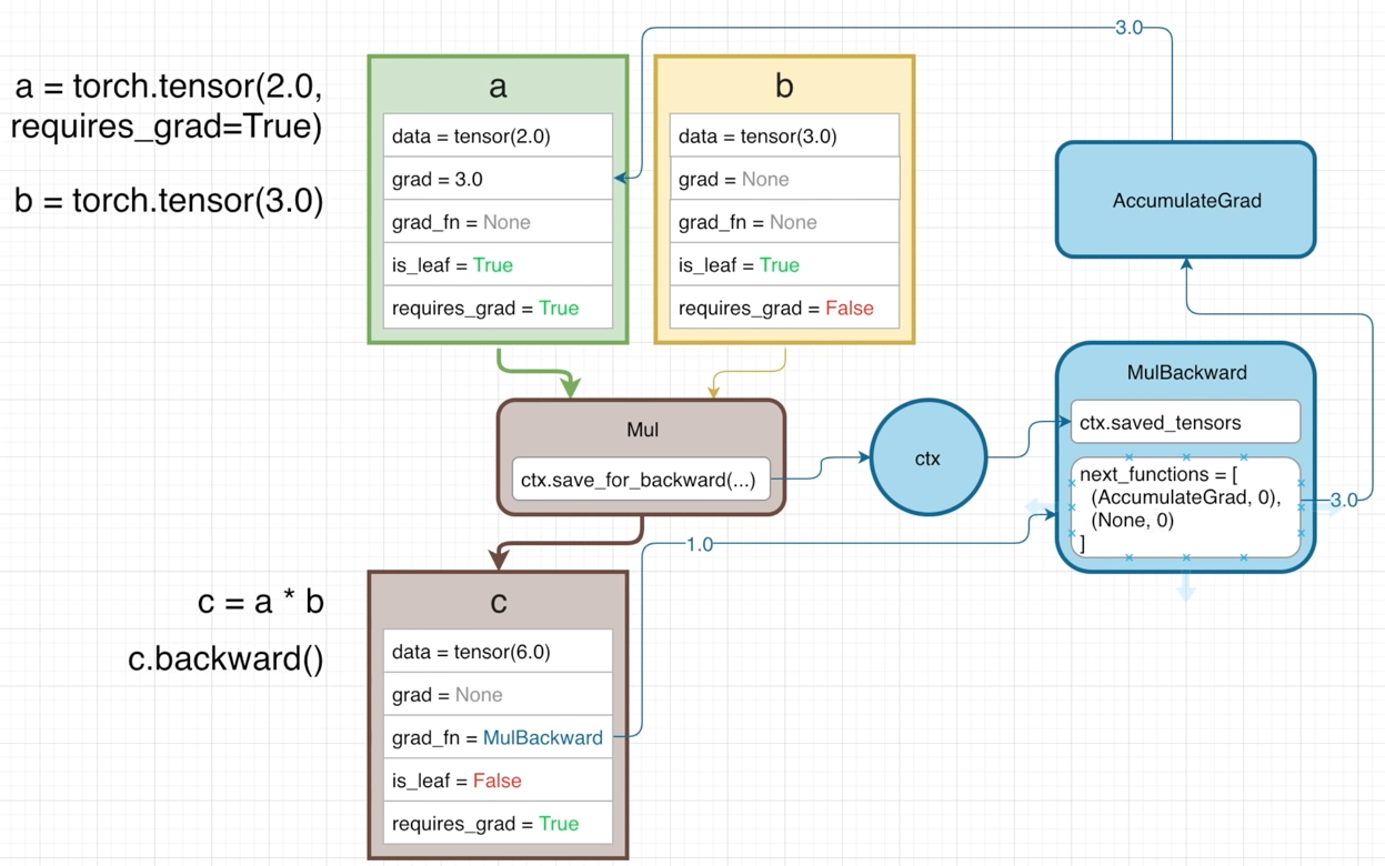
Two tensors are created with the values of 2 and 3 and assigned to variables a and b.
Then the product of a and b is assigned to variable c.
In the following diagram, each struct is a tensor containing several attributes.

dataholds the data of the tensorgradholds the calculated gradient valuegrad_fn, gradient function points to a node in the backwards graphis_leafmarks is this tensor a leaf of a graphrequires_gradis False by default for all tensors that are being input (like a,b) into or output (like c) from an operation. Such that no backwards graph will be created.
However, if the attribute requires_grad of a is set to True and a is passed into any operation (Mul),
the output tensor (c) will also have requires_grad=True and be apart of the backwards graph,
because c is no longer a leaf.
And c’s grad_fn points to MulBackward, which calculates the gardient of its operation w.r.t. input tensor a: ∂c/∂a = ∂(a∗b)/∂a = b

The blue contents are the backwards graph behind the tensors and their operations.

-
When the
Mulfunction is called, thectxcontext variable will save the values to be used in the backwards pass:MulBackwardoperation. -
Specifically, the input tensor
ais stored by the methodctx.save_for_backward(...)and referenced by the propertyctx.saved_tensorsin the backward pass. -
The
MulBackwardhas another attributenext_functionsis a list of tuples, each one associated with an input tensor that were passed to theMuloperation.(AccumulatedGrad, 0)corresponds to the input tensorameaning the gradient ofawill be calculated continuously byAccumulatedGradoperation.(None, 0)is associated with input tensorb, no further calculation is needed for its gradient.
-
The
AccumulateGradoperation is used to sum the gradients (from multiple operations) for the input tensora.
When executing c.backward(), the backward pass of gradients starts. The initial gradient is 1.0 and then passed into MulBackward, where it times b getting 3.0.
Then by looking at the next_functions, it needs to get into AccumulatedGrad to obtain the gradient w.r.t. tensor a.
Finally, the attribute grad of a comes from AccumulateGrad.

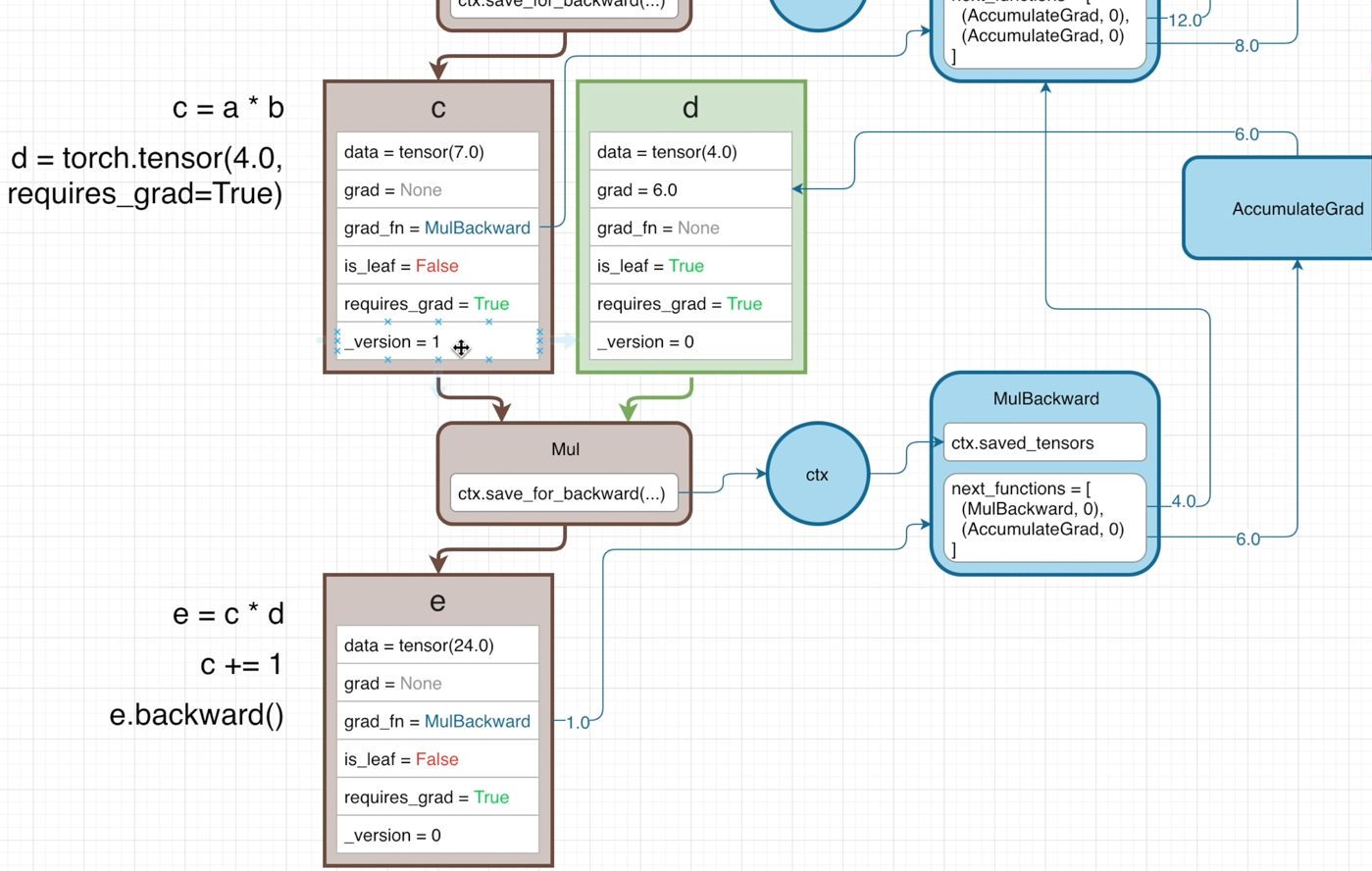
Simple example
Two input tensors are both requires_grad=True.

They’re multiplied together to get c.

If here executing c.backward(), the initial gradient 1.0 will start the backward pass from its grad_fn.

Then tensor d is created to multiply with c to get e.

If executing e.backward() here, to calculate the gradient of e w.r.t. the leaft nodes on the graph,
the backward pass is as follows:

-
The initial gradient 1.0 is first passed into
e.grad_fn, i.e.,MulBackward, where it multiplies with gradient of the operation w.r.t. the leaf nodes: ∂(c∗d)/∂d (=c=6.0).
(Sincecis not a leaf, ∂e/∂c doesn’t need to compute.) -
Then by looking at property
next_functions, the gradients go continuously intoMulBackwardandAccumulateGradseparately.- In
MulBackward, to get ∂e/∂a, the incoming gradient ∂e/∂c multiplies with gradient of theMuloperation w.r.t.a: ∂(a∗b)/∂a, so the gradient of leafais ∂e/∂a = ∂e/∂c × ∂(a∗b)/∂a = 4×3=12.
Also to get ∂e/∂b, the incoming gradient ∂e/∂c multiplies with ∂(a∗b)/∂b, ∂e/∂b = ∂e/∂c × ∂(a∗b)/∂b = 4×2 = 8 - While ∂e/∂c gets into
AccumulateGrad, no other operations needed to calculate the gradients w.r.t. d, thegradof leaf nodedis 6.0.
- In
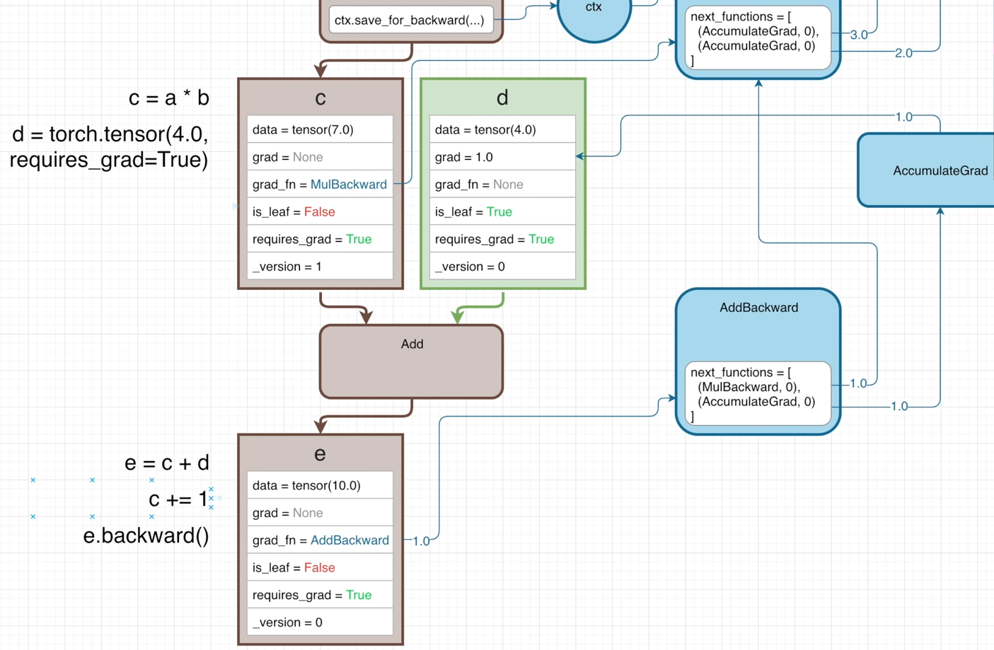
Avoid In-place operation
When the MulBackward operation retrieve input tensors through ctx.saved_tensors, it is necessary to ensure that the correct values are referenced.
Therefore, each tensor must maintains its attribute _version, which will be increamented (+1) when performing in-place operation (e.g., c+=1) each time.

Thus, if calling e.backward() after c+=1, the ctx.saved_tensors will get an error, beacuse the attribute _version of the input tensor c is not matched with the previously saved one.
In this way, the input tensors to be used are ensured haven’t changed in the time since the operation was performed in the forward pass.
However, the Add function doesn’t affect the graidents, so it doesn’t need to save any its input tensors for the backward pass.
Hence, the ctx will not store its input tensors.
And the initial gradient will directly looking at the next_functions after getting into AddBackward node.
In this case, doing c+=1 before e.backward(), no errors will occur because the input tensor c is not retrieved by ctx.saved_tensors.

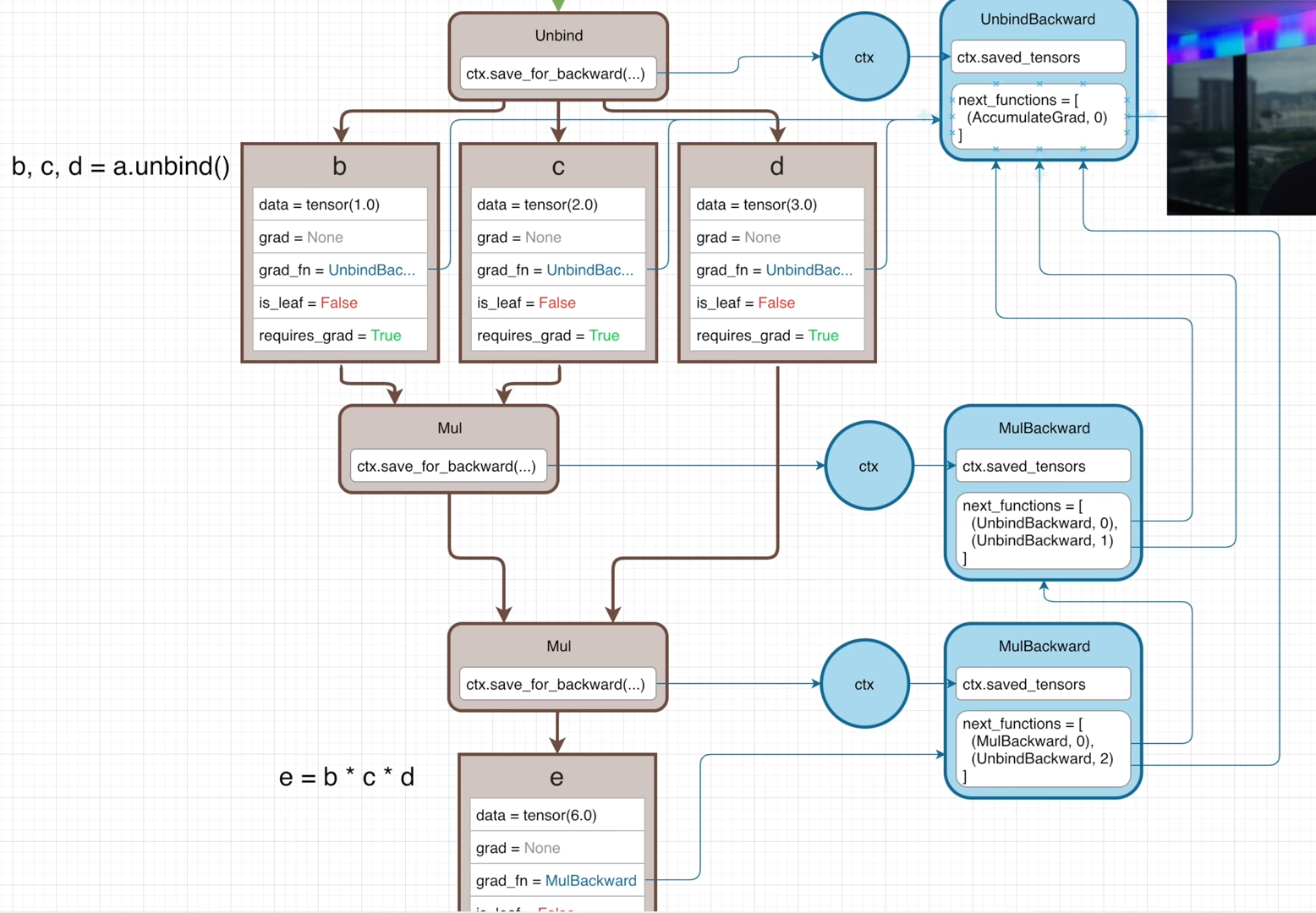
Unbind operation
A tensor is created with 1-D list holding 3 values and assigned to variable a.

Then by executing b,c,d = a.unbind(), tensor a is split along the 1st dimension and tensors b, c, d are created.
This operation will generate the graph as follows:

All of the grad_fn of b, c, d point to the same UnbindBackward function.
If b, c, d are multiplied together to get e, there will be two Mul operation in the forward pass and two MulBackward is the backward pass.

The property next_functions of those 2 MulBackward functions both have tuple (UnbindBackward, i ), but their indecies are different, where i is 0, 1, 2 corresponding to the 3 outputs from the Unbind function.
(UnbindBackward, 0) means the current gradient is associated with the first input tensorbof the (1st)Muloperation, which is also the first output from theUnbindfunction.(UnbindBackward, 1)is saying this is the gradient for the second output fromt heUnbindfunction.(UnbindBackward, 2)indicates this gradient is for the third output of theUnbindfunction.
The index value is used to inform the UnbindBackward which output tensor the gradient is calculated for. Such that the UnbindBackward can output a list of gradients.
The gradient of the leat node can be calculated by calling e.backward(). The backward pass is started off with the initial gradient of 1.
Complicated example
The following scalar tensor can be replaced with any vector or matrix or any n-dimension array.
The tensors are created with the same value of 2 and they both don’t require grad.

a and b are multiplied together to get c, which doesn’t require grad too.

Then by executing c.requires_grad = True, the tensor c will be a port of the backwards graph.
So that any future operations done using c as an input will start to build the backwards graph.
The full forward graph is build as:
- Another tensor
dis created withrequires_grad=False. - Multiply
dwithcto gete. - Another leaf
fis constructed withrequires_grad=False(not on the graph). - Multiply
fwitheto getg - Another tensor
his created withrequires_grad=True(a leaf on the graph). - Devide
gbyhto geti; - Add
iandhtogether to getj. (h is leaf and fed into 2 operations, so itsAccumulteGradhas two inputs fromDivBackwardandAddBackward. - Multiply
janditogether to getk. (i is passed into bothAddandMul, so its (grad_fn)DivBackwardhas 2 streams fromAddBackwardandMulBackward.
Unlikehhas its 2 backward streams converge atAccumulateGrad, the 2 backward streams ofiinstead converge at theDivBackwardthat corresponds to the operationDivgenerating thei.
 (Yellow means the leaf that doesn’t on the graph. Green means the leaf on the graph. Brown means the non-leaf)
At the end, by executing k.backward(), the backward pass will start with a gradient of 1.0, which will times the gradient of each operation w.r.t. local input tensors sequentially from bottom to top.
If an operation’s input is a leaf, the next_functions will point to the AccumulateGrad for this leaf node. Once all gradients streams are accumulated, the sum is put into the attribute grad of the left node.
Finally, ∂k/∂leaf will obtained.

retain_grad()
By default, the gradients will only calculated for the leaf nodes, and the grad of the intermediate nodes are kept None.
But an intermediate tensor can retain their gradient by calling its retain_grad() method.
For example, i.retain_grad(), which will set up a hook
“that gets called in the backward pass that will basically tell the DivBackward function that any gradients passed into it should be saved on the grad attribute of tensor i.

detach()
m = k.detach() will create a new tensor sharing the same underlying data as k, but m will no longer require gradients. m will be a leaft node but not on the graph because its grad_fn is None without pointing any node on the graph.

Usually, the backwards graph is expected to get garbage collected after finishing the training loop.
Once the k.backward() is executed, some values have no references (get freed) in the graph.
Specifically, the references to the saved_tensors.
But the actual graph still exists in memory.
If the output tensor k is needed to kept for longer than the training loop, k can be detached from the graph.
Similar functions:
k.numpy(): ndarrayk.item(): python int or python floatk.tolist(): original tensor that holds multiple values will be converted to python list
(old summary on 2022-10-19)
Those tensors whose attribute requires_grad=True will be nodes on a backwards graph.
Any output tensor yielded from any operation is not leaf node.
grad_fn & grad
The grad_fn of the ’non-leaf’ (intermediate) node points to a node (like MulBackward) which will multiply the incoming gradient by the gradient of this operation w.r.t. its inputs (leaf nodes with requires_grad=True),
or pass the grad of the ’non-leaf’ node up to next gradient-computing node for other leaf nodes before.
This’s like the divergence of ∂L/∂wᶦ and ∂L/∂wᶦ⁻¹.
If an “non-leaf” node is passed into multiple operations, its gradient equals the sum of the gradients coming from each operation. Its gradient will be fed into the “gradient-computing” node as the incoming gradient of the operation that generates it.
While if a leaf node is used by multiple functions, its gradient equals to the sum of the gradients comeing from the “gradient-computeing” nodes of every operation.
Hence, the grad of the leaf node is accumulated by AccumulateGrad function.
ctx
ctx (context) stores the operators doing the operation for computing the gradient in backward graph.
The gradients at different time are different, so the version of variables needs to be recorded.
The in-place operation will increment the version of the variable, and then calling the backward method will cause an error due the mismatch of the _version value.
However, if an operation doesn’t bring gradients (like Add), its operators are not necessary to store. The incoming gradient will not change when passing through its corresponding backwards function (AddBackward).
In this case, modifying its operators before calling .backward() is okay, becaue they are not involved with gradient.
Gradient for a one-dim tensor is a list of partial derivative. The second value in the tuple is the index among the mutliple outputs of the operation, indicating to who the gradient belongs
output don’t have grad by default
The “non-leaf” node will not store grad by default, unless set its .retain_grad(), from which a hook can be set up to make its grad_fn to save any gradient passed to it into grad of this node.
detach()
m=k.detach() will create a leaf node m sharing the same data as k, but will no longer require gradient. Its grad_fn=None meaning it doesn’t have a reference to the backwards graph. This operation is used to store a output value separately, but free the backwards graph after a training loop (forward+backward).
Alternatives for detaching from the graph:
k.numpy(),k.item()convert one-element tensor to python scalar.k.tolist().
(2022-11-01)
gradientis the upstream gradients until this calling tensor (from the intermediate node to the network ouput).
Since the explicit expression of output is unknown, the derivative $\rm\frac{ d(output) }{ d(input) }$ cannot be calculated directly. But the derivative $\rm\frac{ d(output) }{ d(intermediate) }$ and $\rm\frac{ d(intermediate) }{ d(input) }$ are all known. Therefore, by passing the d(output)/d(intermediate), say 0.05, togradient, the d(output)/d(input) is the returned value ofintermeidate.backward(gradient=0.05,). The gradient argument in PyTorch backward - devpranjal Blog
(2023-08-02)
Freeze params
-
module.requires_grad_(False)will change all its parameters. PyTorch Forum-
If I explicitly add the learnable params one-by-one, like this tutorial (
if p.requires_grad), only the ordinal of the layers in the state dictckpt['optimizer]['state']changed, while the total number of states remains the number of layers to be performing gradient descent.1 2 3 4 5 6 7# Test in GNT with multiple encoders: self.optimizer.add_param_group({"params": self.multiEncoders.parameters()}) # Saved `ckpt['optimizer']['state']` has a max index: 1390, but total 262 layers. params = [p for p in self.multiEncoders.parameters() if p.requires_grad] self.optimizer.add_param_group({"params": params}) #`ckpt['optimizer']['state']` has a max index: 281, but total 262 layers too.
-
-
with torch.no_grad():will stop backward-propagation for a block of operations wrapped in its region (in a context). This is equivalent tomodule.requires_grad_(False). Demo-SO- Inference mode is similar with
no_grad, but even faster.
- Inference mode is similar with
-
module.eval()=module.train(False)affects the settings ofnn.Dropoutandnn.BatchNorm2d. And it has nothing to do withgrad. Docs - Autograd- In pixelNeRF,
self.net.eval()andself.net.train()will jump toSwinTransformer2D_Adapter.train(mode=True)
- In pixelNeRF,
requires_grad_ vs requires_grad
requires_grad_ can do for non-leaf node, while requires_grad will have error.
PyTorch Forum
Twice nn.Parameter
(2024-04-11)
|
|
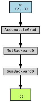
As shown above, once “re-convert” the w@x as the nn.Parameter,
the forward graph doesn’t include w and the operation Matrixmultiplication.
The graph is starting from f instead.
Therefore, even though w is a leaf node and require_grad is True, it won’t obtain .grad: w.grad is None.
In contrast, do not re-set the nn.Parameter won’t change the leaf tensors.
|
|
In this way, the leaf tensors are prepared outside the for loop (specifally forward()).
And the leaf tensors (i.e., w) will be added onto the graph correctly during each iteration rebuilding.
Graph in For Loop
(2024-04-11)
The computational graph (of PyTorch 1.x) is build in each iteration,
as the previous graph has been destroyed after executing .backward()
Therefore, the tensors to be optimized, i.e., the leaf node of the graph, have to be present within the for loop as the starting point of the graph.
In the following code, w needs to be optimized.
|
|
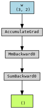
The forward graph can be plotted as:
- The endpoint (green box) is the tensor
loss - The
whas performed Multiplication and Sum to getloss - The graph will be rebuilt in each iteration, with the
wandxas the starting points. And the graph will be freed afterloss.backward() optimizer.step()updates leaf tensors that require grad. Docs
Code
|
|
However, if moving the operation f=w*x outside the for loop,
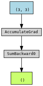
the graph only contain an operation: f.sum()
|
|
From the second run, the rebuilt graph only includes “Sum”, and no longer includes w (out of this graph).
In other words, the w doesn’t belong to this newly rebuilt graph.
Therefore, the .backward() method cannot be completed for w.
In the second iteration, the graph doesn’t include w. So, when the gradient backpropagates, the gradient cannot reach w.
On the other hand, the w still points to the previous graph, without updating.
Error:
|
|