Code-pytroch | Arxiv | OpenReview
Q&A
- Condition image vs target image?
Abstract
-
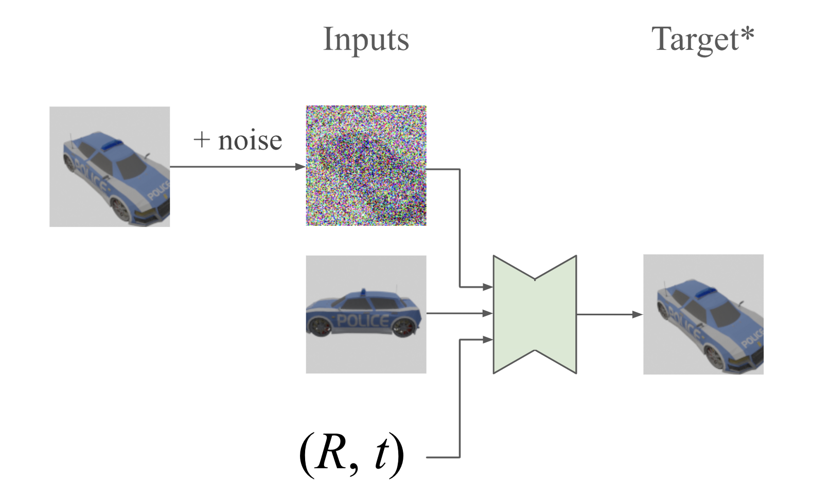
A img2img diffusion model is conditioned with pose and a single source view to generate multiviews.
-
Stochastic conditioning: Randomly select a view from avaliable views as condition image at each denoising step during sampling?, rather than using only the given view.
-
Reconstruct a NeRF to measure 3D consistency of multi-views.
- NeRF is not their ultimate objective.
Intro
-
Regressive methods for NVS from sparse views based on NeRF are still not generalizable enough or able to produce high-quality completion for the occluded parts.
-
Regularized NeRF (RegNeRF) suffer from artifacts when only few views are given
because theyand didn’t apply the features of commen prior of multiple scenes. -
Regressing a NeRF from image feataures (pixel-NeRF) tend to get blurred images.
-
-
Geometry-free methods for NVS obtain colors that aren’t directly derived from volume rendering.
- Light field network
- Scene Representation Transformer
- EG3D combines StyleGAN and volume rendering
-
3D diffusion model is a generative and geometry-free method.
- Use pairs of images of the same scene to train a diffusion model.
- During training, one of them serves as the original, and the other is the condition image.
- The trained model can produce a multi-view set of a scene given one condition image.
Model
They consider multiple views from a scene are not independent, but follow the distribution of the training views, to enhance multi-view consistency.
-
The distributions of different views, given a scene with a total observation set 𝐒, $p(𝐱|S)$ are conditionally independent (different).
-
NeRF solves NVS under an even strict condition: each ray in the scen is conditionally independent.
-
However, with this nature, the diffusion model cannot guarantee the samplings (generated images), conditioned with different source view, follow a common distribution, i.e., the diffusion model needs a unique distribution to learn.
Ideally, the common distribution should be p(S), but it’s difficult to approximate the entire scene based on sparse views. (Not sure, my guess.)
That’s why they reused the generated views previously for later condition.
Pose-conditioned
Given the data distribution p(𝐱₁, 𝐱₂), diffusion model learns the distribution of one of the two images conditioned on the other image and both poses.
- Noise schedule involving signal-to-noise ratio λ.
- Loss function of DDPM
Stochastic condition
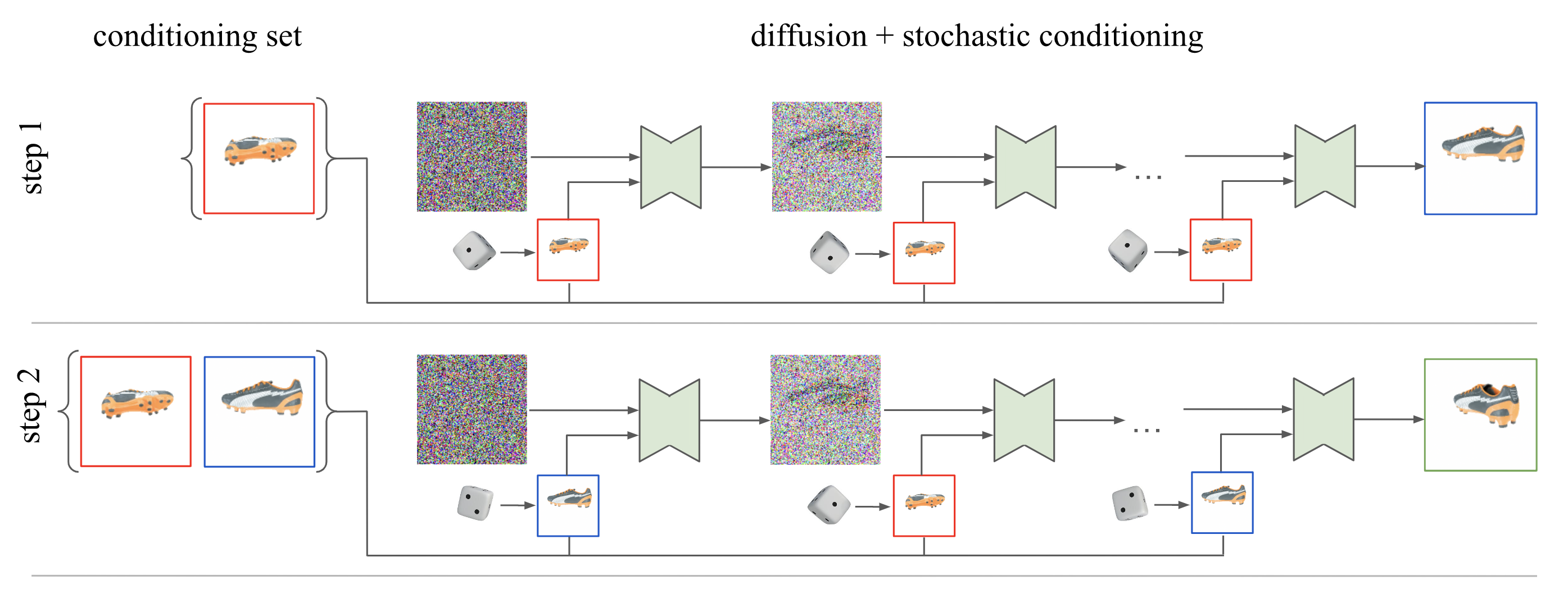
Figure 3: Stochastic conditioning sampler
-
Markovian model didn’t perform well, where the next image is conditioned on (k) previously generated views. Thus, a scene can be represented as $p(𝐗) = ∏ᵢp(𝐱ᵢ|𝐱_{<i})$.
-
Using all previous sampled views is imfesible due to the limited memory.
-
They found k=2 can achieve 3D consistency, but more previous states impair the sampling quality.
-
And instead of conditioning on the last few samplings as in the Markovian model, 2 views are stochastically selected as condition images at each denoising step.
-
-
Generating a new view $𝐱ₖ₊₁$ needs 256 denoising steps, where each time the condition image 𝐱ᵢ is randomly chosen from the current views set 𝜲 = {𝐱₁,…,𝐱ₖ}.
-
In a denoising step, noise in the intermediate image $\hat 𝐱ₖ₊₁$ will be subtracted from $𝐳ₖ₊₁^{(λₜ)}$, which follows a forward noising distribution 𝒒, given the noisy image $𝐳ₖ₊₁^{(λₜ₋₁)}$ of last step and the denoised image $\hat 𝐱ₖ₊₁$.
$$ \hat 𝐱ₖ₊₁ = \frac{1}{\sqrt{σ(λₜ)}} \left( 𝐳ₖ₊₁^{(λₜ)} - \sqrt{σ(-λₜ)}\ ε_θ(𝐳ₖ₊₁^{(λₜ)}, 𝐱ᵢ) \right) \\ \ \\ 𝐳ₖ₊₁^{(λₜ₋₁)} \sim q(𝐳ₖ₊₁^{λₜ₋₁};\ 𝐳ₖ₊₁^{(λₜ)}, \hat 𝐱ₖ₊₁ ) $$
-
( I guess 𝒒 gets “reversed” after applying Bayes rule)
-
The first noisy image $𝐳ₖ₊₁^{(λ_T)}$ is Gaussian N(0,𝐈).
-
-
After 256 steps finished, add the result image 𝐱ₖ₊₁ to set 𝜲.
-
256 can be larger to cover all the existing views.
-
This scheme approximate the true autoregressive sampling.
-
Autoregressive model always use all previous states to predict the next state, unlike Markov chain only considering limited recent outputs,
Therefore, to train an autoregressive model, a sequence, i.e. multi-view training data here, is needed.
“True autoregressive sampling needs a score model of the form $log\ q(𝐳ₖ₊₁^{(λ)} | 𝐱₁,…,𝐱ₖ)$ and multi-view training data.”
-
But they’re not interesting in multiple source views here.
-
-
X-UNet
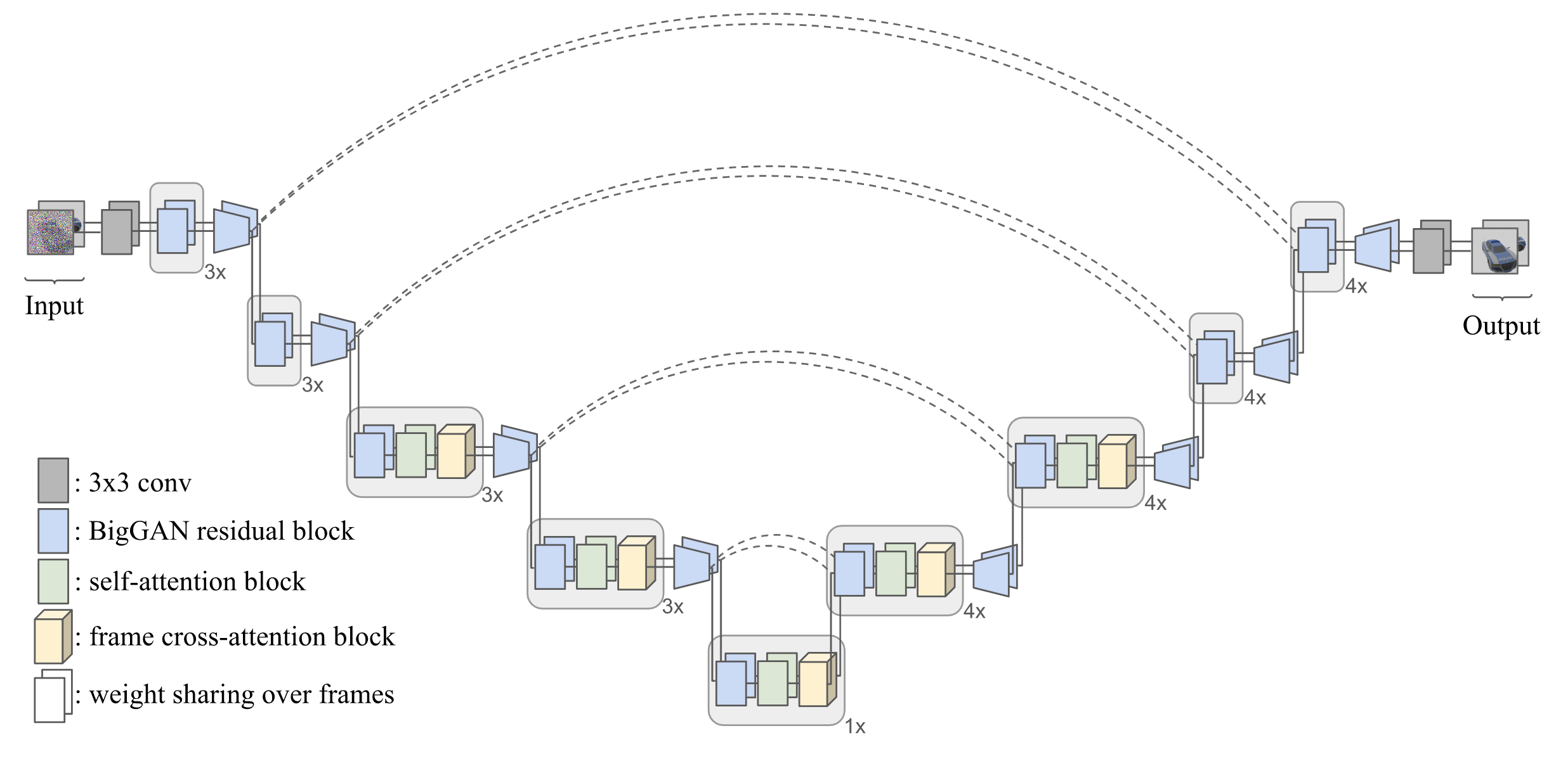
Figure 4: X-UNet Architecture
UNet with only self-attention fails to generate images with multi-view consistency, given limited training images.
- Different frame has a different noise-level
- Positional encoding of pose is the same size of feature maps
- Use cross-attention to make two images attend to each other.
Inputs:
Concat two images? such that the weights of Conv2d and self-attention layers are shared for the noisy image and condition image
Experiments
Dataset: SRN ShapeNet (synthetic cars and chairs) github
| file | size |
|---|---|
| cars_train.zip | 3.26GB |
| chairs_train.zip | 60.3GB |
Use instant-NGP without view dependent modules