Code | arXiv | Vickie Ye

• Surfaced by NeRF&Beyond 12.5日报(CustomNeRF，VideoRF，网格引导编辑，SANeRF-HQ，GPS-Gaussian，两个GaussianAvatar，SpalTAM，gsplat） - Jason陪你练绝技的文章 - 知乎
  
• Feature image from: Understanding the Covariance Matrix - Janakiev

Projection

NDC Mapping

(2024-01-01)

The perspective division (a 3D pixel coordinates are divided by the 3rd dimension) should be performed as the final step in the transformation pipeline, as it’s a non-linear operation.

Given a 3D point (x,y,z)ᵀ located in the camera space, the perspective projection and scaling are carried out in sequence to obtain its clip coordinates (not NDC yet).

$$ \begin{array}{c} \text{[Scaling Matrix] [Perspective Projection] [Camera space] = [Clip space]} \\ \\ \begin{bmatrix} □ & □ & □ & □ \\ □ & □ & □ & □ \\ □ & □ & □ & □ \\ □ & □ & □ & □ \end{bmatrix} \begin{bmatrix} fₓ & 0 & cₓ & 0 \\ 0 & f_y & c_y & 0 \\ 0 & 0 & 1 & 0 \\ 0 & 0 & 0 & 1 \\ \end{bmatrix} \begin{bmatrix} x \\ y \\ z \\ 1 \end{bmatrix} = \begin{bmatrix} x_c \\ y_c \\ z_c \\ w_c \end{bmatrix} \end{array} $$

The scaling matrix is built with the goal of mapping the view frustum to a [-1,1] NDC-space cube encompassing only valid points, whose clip coordinates satisfy: $-w_c < x_c,y_c,z_c < w_c$. Specifically, the projected coordinates are scaled and then perform perspective division to become the NDC.

1. Perspective projection:

   $$ \begin{bmatrix} fₓ & 0 & cₓ & 0 \\ 0 & f_y & c_y & 0 \\ 0 & 0 & 1 & 0 \\ 0 & 0 & 0 & 1 \\ \end{bmatrix} \begin{bmatrix} x \\ y \\ z \\ 1 \end{bmatrix} = \begin{bmatrix} fₓx + cₓ z \\ f_y y + c_y z \\ z \\ 1 \end{bmatrix} $$

2. Scaling projected coordinates u and v to [-1, 1]

   To scale u, the 1st row of the scaling matrix is A 0 B 0.

   Perform scaling first, followed by perspective division, to obtain the x in NDC space: $\frac{A (fₓ x + cₓ z) + Bz}{z} = A (\frac{fₓ x}{z} + cₓ) + B ∈ [-1,1]$

   Since $(\frac{fₓ x}{z} + cₓ) = u ∈ [0,W]$

   $$ \begin{cases} A0 + B = -1 \\ AW + B = 1 \end{cases} ⇒ \begin{cases} A = \frac{2}{W} \\ B = -1 \end{cases} $$

   Therefore, the first 2 rows are:

   $$ \begin{bmatrix} 2/W & 0 & -1 & 0 \\ 0 & 2/H & -1 & 0 \\ □ & □ & □ & □ \\ □ & □ & □ & □ \end{bmatrix} \begin{bmatrix} fₓx + cₓ z \\ f_y y + c_y z \\ z \\ 1 \end{bmatrix} $$

3. Scaling frustum $z ∈ [n, f]$ to [-1,1]

   z is independent to x and y, so the 3rd row only has 2 unknows: 0 0 A B.

   Scaling first, then perspective division, thereby the z in NDC space is: $\frac{A z + B}{z} ∈ [-1, 1]$

   Substituting z = n and f:

   $$ \begin{cases} \frac{A n + B}{n} = -1 \\ \frac{A f + B}{f} = 1 \end{cases} ⇒ \begin{cases} A = \frac{f+n}{f-n} \\ B = \frac{-2fn}{f-n} \end{cases} $$

   Finally, since the denominators are z (i.e., the w of a point’s clip coordinates is z), the 4th row is 0 0 1 0:

   $$ \begin{bmatrix} 2/W & 0 & -1 & 0 \\ 0 & 2/H & -1 & 0 \\ 0 & 0 & \frac{f+n}{f-n} & \frac{-2fn}{f-n} \\ 0 & 0 & 1 & 0 \end{bmatrix} \begin{bmatrix} fₓx + cₓ z \\ f_y y + c_y z \\ z \\ 1 \end{bmatrix} = \begin{bmatrix} \frac{2 (fₓx + cₓ z)}{W} - z \\ \frac{2 (f_y y + c_y z) }{H} - z \\ \frac{f+n}{f-n} z - \frac{2fn}{f-n} \\ z \end{bmatrix} $$

   The result coordinates are in the clip space, which will become ND coordinates after perspective division, and only points within the cube of [-1,1] in NDC space will be rendered.

In summary, the Projection Matrix (GL_PROJECTION) transforming camera-space (x,y,z)ᵀ to clip coordinates is:

$$ P = \begin{bmatrix} \frac{2}{W} & 0 & -1 & 0 \\ 0 & \frac{2}{H} & -1 & 0 \\ 0 & 0 & \frac{f+n}{f-n} & \frac{-2fn}{f-n} \\ 0 & 0 & 1 & 0 \end{bmatrix} \begin{bmatrix} fₓ & 0 & cₓ & 0 \\ 0 & f_y & c_y & 0 \\ 0 & 0 & 1 & 0 \\ 0 & 0 & 0 & 1 \end{bmatrix} = \begin{bmatrix} \frac{2fₓ}{W} & 0 & (\frac{2cₓ}{W}) -1 & 0 \\ 0 & \frac{2f_y}{H} & (\frac{2c_y}{H}) -1 & 0 \\ 0 & 0 & \frac{f+n}{f-n} & \frac{-2fn}{f-n} \\ 0 & 0 & 1 & 0 \end{bmatrix} $$

• When cx and cy are W/2 and H/2, it’s in the form of Ye’s article.

• When cx and cy are r and t, it’s in the form of songho.

(2024-01-02)

Project mean vector 𝛍

A mean vector 𝛍 in world space is changed to pixel space as follows:

• 𝐭 refers to coordinates of 𝛍 in the camera space as: $𝐭 = \begin{bmatrix} 𝐑_{w2c} & 𝐭_{w2c} \\ 0 & 1 \end{bmatrix} \begin{bmatrix} \bm μ \\ 1 \end{bmatrix}$

  • While the translation vector is denoted as $𝐭_{w2c}$.

  • And the extrinsics is represented as $𝐓_{w2c}$.

  • The clip coordinates of 𝛍 is $𝐭’ = 𝐏𝐭$

  • The nonlinear perspective division is approximated by the projective transformation $ϕₖ(𝐭’)$.

1. Points’ coordinates conversion from world space to clip space:

   $$ \begin{aligned} 𝐭’ &= 𝐏⋅ 𝐓_{w2c}⋅ [^{\bm \mu}_1] \\ &=\begin{bmatrix} \frac{2fₓ}{W} & 0 & (2cₓ/W) -1 & 0 \\ 0 & \frac{2f_y}{H} & (2c_y/H) -1 & 0 \\ 0 & 0 & \frac{f+n}{f-n} & \frac{-2fn}{f-n} \\ 0 & 0 & 1 & 0 \end{bmatrix} \begin{bmatrix} R_{w2c} & t_{w2c} \\ 0 & 1 \end{bmatrix} \begin{bmatrix} μₓ \\ μ_y \\ μ_z \\ 1 \end{bmatrix} = \begin{bmatrix} tₓ’ \\ t_y’ \\ t_z’ \\ t_w’ \end{bmatrix} \end{aligned} $$

   • $t_w’$ is the point’s camera-space depth $t_z$, which is > 0.

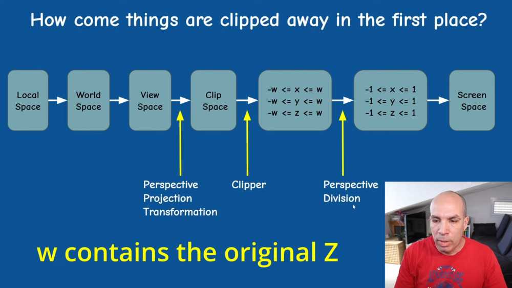
2. Frustum clipping (clip-space culling) filters points that won’t appear in the frustum based on clip coordinates before perspective division:

   View Frustum Clipping - UofTexas - Lec9

   • View frustum clipping aims to reduce computation. Essentially, it filters points by comparing the clip coordinate $w_c$ with $x_c, y_c, z_c$ for each point.

   • In the previous derivation, clip coordinates are the scaled projection coordinates: (A*ProjCoord+B). NDC space is defined by $w$, as the NDC cube is constrained by bounds where the clip coordinates divided by 𝑤 equals 1 (𝑤 is the benchmark), such as $\frac{A (f_x x+c_x z) + Bz}{w} = 1$

     In other words, the NDC planes wrap around points whose clip coordinates $x_c,y_c,z_c$ less than or equal to $w_c$. In addition, $w_c$ must be the camera-space depth z for the final perspective division. Thus, if the clip coordinate of a point is bigger than w or less than $-w$, the “quotient” will be outside of [-1,1], i.e., the point is not located in the camera-space view frustum or the NDC-space cube.

     Frustum clipping retains points that satisfy: $-w_c \leq x_c, y_c, z_c \leq w_c$. Conversely, those points whose w (equals camera-space depth) is smaller than x,y,z will be filtered out.

     Although ND Coordinates are also able to identify points for clipping, to reduce the number of perspective divisions (executed at final), clipping is performed in the clip space for efficiency.

   • On the other hand, since the ND Coordinates of the Left, Right, Bottom, Top, Near, and Far frustum planes are -1 and 1, the clip coordinates of points located within the Frustum satisfy the relation: $-1 < \frac{x_c}{w_c}, \frac{y_c}{w_c}, \frac{z_c}{w_c} <1$

   • Consequently, only points in the frustum (i.e., NDC-space cube: $-1 < xₙ, yₙ, zₙ < 1$) are survived.

   • (2024-01-03) It is the view frustum clipping that makes ND coordinates can be regarded as a cube space, because out-of-the-cube points have been disregared.

3. Performing perspective division on the clip coordinates resulting in NDC, whose all components ranges in [-1,1]:

   $$ NDC = \begin{bmatrix} tₓ’/t_w’ \\ t_y’/t_w’ \\ t_z’/t_w’ \\ 1 \end{bmatrix} ∈ [-1,1] $$

   • (2024-02-08) NDC is 3D, including zₙ coord besides the 2D pixel coords.

4. Scaling NDC to obtain pixel coordinates 𝛍’ (viewport transformation): songho

   $$ [-1, 1] \overset{×W}{→} [-W, W] \overset{+1}{→} [-W+1,W+1] \overset{÷2}{→} [\frac{-W+1}{2}, \frac{W+1}{2}] \\ \overset{+c_x}{→} [0.5, W+0.5] (\text{ if $c_x =\frac{W}{2}$}) $$

   Therefore, the final pixel coordinate 𝛍’ of a world-space mean vector 𝛍 is:

   $$ \bm \mu’ = \begin{bmatrix} (W⋅tₓ’/t_w’ + 1) /2 + c_x \\ (H⋅t_y’/t_w’ + 1) / 2 + c_y \end{bmatrix} $$

Project Covariance

(2024-01-03)

1. Because the perspective projection is not a linear operation due to division, the 2D projection of a 3D Gaussian is not a 2D Gaussian:

   snowball splat diffuse	Is it a 2D Gaussian?	Conic sections

2. EWA Splatting doesn’t scale the projected coordinates to the [-1,1] NDC-space cube. It directly transforms points from camera space onto screen (or viewing-ray space) by dividing z. The result coordinates range in [0,W] and [0,H].

3. Projective transformation ϕ(𝐭) in EWA Splatting: Converting an arbitrary point’s camera-space coordinates $𝐭=(tₓ,t_y,t_z)ᵀ$ to the coordinates in 3D ray space (pixel coordinates x0,x1 + “new depth” x2) has 2 steps:

   • Pixel coords = perspective projection + perspective division.
   • The new depth is set to the L2 norm of the point’s camera-space coordinates.

   $$ ϕ(𝐭) = \begin{bmatrix} \frac{fₓ tₓ}{t_z} + cₓ \\ \frac{f_y t_y}{t_z} + c_y \\ \sqrt{t_x^2 + t_y^2 + t_z^2} \end{bmatrix} = \begin{bmatrix} x_0 \\ x_1 \\ x_2 \end{bmatrix} $$

   Because EWA Splatting doesn’t consider frustum clipping, the approximation is based on the camera coordinates 𝐭.

   • (2024-02-16) The clip coordinates shouldn’t be used in EWA splatting because the Gaussian center is used in the Jacobian that approximates the perspective projection, where the camera-space coordinates are supposed to be used.

     Whereas, 3DGS (or gsplat) requires to determine whether the point (Gaussian center) is in the frustrum to be rendered, the clip coordinates are utilized for frustum clipping. Therefore, the world coordinates 𝐱 are involved into 2 procedures: the covertion for covariance matrix from world space to ray space (JW𝚺WᵀJᵀ), and the projection for Gaussian center from world space onto the screen.

     Consequently, the derivative of Loss w.r.t. the world coordinates ($\frac{∂L}{∂𝐱}$) has 2 portions.

   However, gsplat uses the clip space to filter points outside the camera frustum. So, after perspective projection and scaling for NDC with matrix 𝐏, points are transferred into clip space as 𝐭’ for clipping.

   After clipping, the nonlinear perspective division and x₂ reassignment in ϕ(𝐭), are approximated with an affine transformation based on the clip coordinates 𝐭’. Therefore, the projective transformation $ϕ(𝐭)$ that maps camera space to ray space becomes a mapping from clip space to the ray space $ϕ(𝐭’)$.

   $$ \begin{aligned} 𝐭 &→ 𝐭’=𝐏𝐭 = \begin{bmatrix} \frac{2 (fₓ t_x + cₓ t_z)}{W} - t_z \\ \frac{2 (f_y t_y + c_y t_z) }{H} - t_z \\ \frac{f+n}{f-n} z - \frac{2fn}{f-n} \\ t_z \end{bmatrix} = \begin{bmatrix}𝐭_x’ \\ t_y’ \\ t_z’ \\ t_z\end{bmatrix} \\ &→ ϕ(𝐭’) = \begin{bmatrix} tₓ’/t_z’ \\ t_y’/t_z’ \\ ‖𝐭’‖₂ \end{bmatrix} = \begin{bmatrix} x_0 \\ x_1 \\ x_2 \end{bmatrix} \end{aligned} $$

   The affine approximation is the first 2 terms of $ϕ(𝐭’)$’s Taylor expansion evaluated at a Gaussian’s mean vector $𝐭ₖ’ = (t_{k,x}’, t_{k,y}’, t_{k,z}’)ᵀ$ in the clip space:

   $$ \begin{aligned} & ϕ(𝐭’) ≈ ϕₖ(𝐭’) = ϕ(𝐭ₖ’) + 𝐉_{𝐭ₖ’} ⋅ (𝐭’ - 𝐭ₖ’) \\ & = \begin{bmatrix} t_{k,x}’/t_{k,z}’ \\ t_{k,y}’/t_{k,z}’ \\ ‖𝐭ₖ’‖²\end{bmatrix} + \begin{bmatrix} 1/t_{k,z}’ & 0 & -t_{k,x}/{t_{k,z}’}^2 \\ 0 & 1/t_{k,z}’ & -t_{k,y}/{t_{k,z}’}^2 \\ t_{k,x}’/‖𝐭ₖ’‖₂ & t_{k,y}’/‖𝐭ₖ’‖₂ & t_{k,z}’/‖𝐭ₖ’‖₂ \end{bmatrix} (𝐭’ - 𝐭ₖ’) \end{aligned} $$

   ---

   If using the camera-space coordinates 𝐭 to express the projective transformation as ϕ(𝐭), focal lengths will be exposed:

   $$ \begin{aligned} ϕ(𝐭) ≈ ϕₖ(𝐭) &= ϕ(𝐭ₖ)+ 𝐉_{𝐭ₖ} ⋅ (𝐭 - 𝐭ₖ) \\ &=\begin{bmatrix} 2(fₓ t_{k,x}/t_{k,z} + cₓ)/W -1 \\ 2(f_y t_{k,y}/t_{k,z} + c_y)/H -1 \\ ‖𝐭ₖ‖₂ \end{bmatrix} + 𝐉_{𝐭ₖ} ⋅ (𝐭 - 𝐭ₖ) \end{aligned} $$

   If $c_x=W/2,\ c_y=H/2$, then $ϕₖ(𝐭) = \begin{bmatrix} \frac{2f_x t_{k,x}}{W⋅ t_{k,z}} \\ \frac{2f_y t_{k,y}}{H⋅ t_{k,z}} \\ ‖𝐭ₖ‖₂ \end{bmatrix}$

   and the Jacobian $𝐉_{𝐭ₖ}$ will be:

   $$ 𝐉_{𝐭ₖ} = \begin{bmatrix} (2/W)⋅fₓ/t_{k,z} & 0 & (2/W)⋅-fₓ t_{k,x} / {t_{k,z}}^2 \\ 0 & (2/H)⋅f_y/t_{k,z} & (2/H)⋅-f_y t_{k,y} / {t_{k,z}}^2 \\ t_{k,x}/‖𝐭ₖ‖₂ & t_{k,y}/‖𝐭ₖ‖₂ & t_{k,z}/‖𝐭ₖ‖₂ \end{bmatrix} $$

   • If the camera-film coords x∈[0,W] and y∈[0,H] are not scaled to [-1,1], the scaling factors 2/W and 2/H won’t exist.

     Thus, the Jacobian evaluated at center 𝐭ₖ in the camera space is:

     $$ 𝐉_{𝐭ₖ} = \begin{bmatrix} fₓ/t_{k,z} & 0 & -fₓ t_{k,x} / {t_{k,z}}^2 \\ 0 & f_y/t_{k,z} & -f_y t_{k,y} / {t_{k,z}}^2 \\ t_{k,x}/‖𝐭ₖ‖₂ & t_{k,y}/‖𝐭ₖ‖₂ & t_{k,z}/‖𝐭ₖ‖₂ \end{bmatrix} $$

   • By expressing the projective transformation ϕₖ() with the camera coordinates 𝐭, the relation between ray-space coordinates and camera-space coordinates is constructed. Thereby, the derivative of Gaussian center ϕₖ(𝐭ₖ) in the ray space is derived from camera-space coordinates 𝐭ₖ, with the clip coordinates 𝐭ₖ’ skipped.

   For the case of 2D projection, only x and y dimensions of the covariance matrix need consideration, with the 3rd row and column are omitted. Because of the affine approximation, the projective transformation ϕ(𝐭’) becomes a linear operation. Thereby, a 3D Gaussian after perspective division is a 2D Gaussian.

   • Figuratively, points surrounding the 3D Gaussian center in clip space will fall into an ellipse on the 2D screen.
   • In the 3DGS code, the 2D ellipse is further simplified as a circle to count the overlapped tiles.

4. The covariance matrix 𝚺ₖ’ of the 2D Gaussian in the pixel space corresponding to the 3D Gaussian (𝚺ₖ) in the world space can be derived based on properties of Gaussians as:

   $$\bm Σₖ’ = 𝐉ₖ 𝐑_{w2c} \bm Σₖ 𝐑_{w2c}ᵀ 𝐉ₖᵀ$$

5. Because covariance matrix 𝚺’ is symmetric, it can be decomposed to a stretching vector (diagonal matrix) and a rotation matrix by SVD, analogous to describing the configurations of an ellipsoid ^3DGS. (Essentially, the covariance matrix depicts a data distribution.)

   The rotation matrix is converted to a quaternion during optimization.

In summary: A 3D Gaussian (𝛍ₖ,𝚺ₖ) in world (object) space is transformed into 3D ray space (or the screen with the 3rd dim omitted), resulting in:

• Mean vector: $\bm μₖ’ = ϕ(𝐭ₖ’)$, where $𝐭ₖ’ = 𝐏⋅ [^{𝐑_{w2c} \ 𝐭_{w2c}}_{0 \quad\ 1}] ⋅[^{\bm μₖ}_1]$ is clip coordinates.

• Covariance matrix: $\bm Σₖ’ = 𝐉ₖ⋅ 𝐑_{w2c}⋅ \bm Σₖ⋅ 𝐑_{w2c}ᵀ⋅ 𝐉ₖᵀ$

• A point 𝐭’ in clip space within the Gaussian distribution is projected to ray space: $ϕₖ(𝐭’) = ϕ(𝐭ₖ’) + 𝐉ₖ⋅(𝐭’ - 𝐭ₖ’)$. The discrepancy between the approximated and the real projected locations is $ϕₖ(𝐭’)-ϕ(𝐭’)$.

Rasterizing

Sorting Kernels

(2024-01-09)

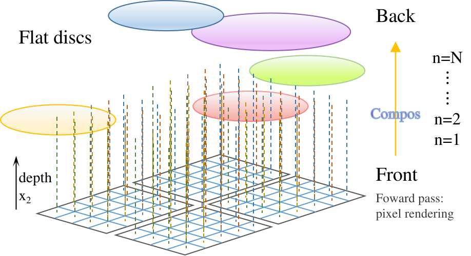
Sort Gaussians within each 16x16 tile based on depth

• Every pixel has a perpendicular dot line, and the discs intersected with the line are visible to the pixel.

• The depths of those discs are $x₂ = ‖𝐭’‖₂ = \sqrt{ {t₀’}² + {t₁’}² + {t₂’}²}$, L2 norm of the clip coordinates.

• The disc closer to the screen is more prominent.

• Different images are obtained given different viewing rays, as the opacities of the discs change in tandem with viewing rays. (Specifically, the opacity of a disc is an integral for the Gaussian in the 3D ray space along a viewing ray.)

  In contrast, volume rendering method changes point-wise colors on different viewing rays.

• (2024-01-22) In splatting, image formation still relies on alpha compositing. Distinct from NeRF where a pixel-ray originates from the camera optical center, in splatting, a pixel emits a perpendicular ray from the screen. And it is the incoming viewing rays determine varying alpha (opacity) of the filters on the pixel-ray path. Such that the screen displays diverse colors with various viewing rays.

  (2024-04-20)

  • I think the “screen” is indeed the camera film. The “viewing ray” doesn’t hit the screen". The viewing ray is just required to pass through 3D Gaussians to calculate each Gaussian’s opacity by integrating the 3D Gaussian over the intersecting segment.

    Rendering a pixel in the splatting method also emitting a ray from a pixel and compositing discs on the ray. The difference is that the opacity has been precomputed by splatting procedure: integrating the viewing ray.

    Thus, it is the screen, i.e., pixels that shoot lines.

    

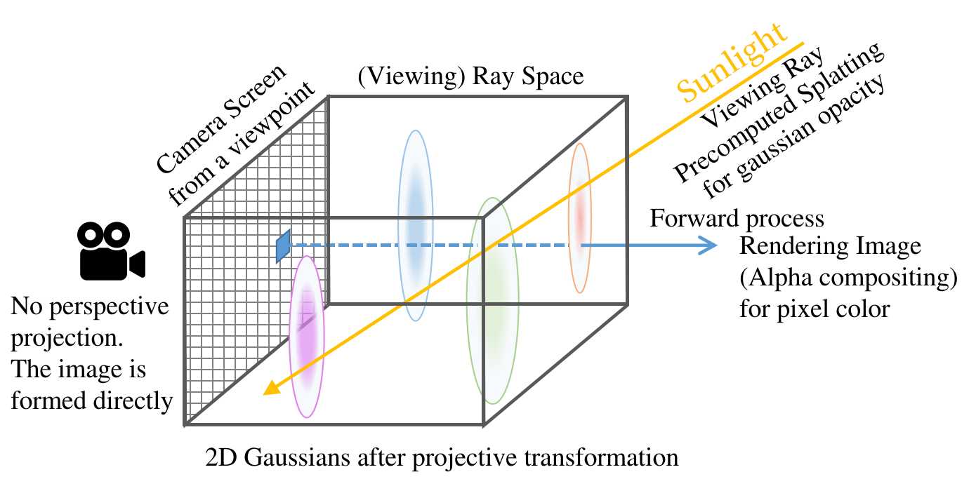
    In the implementation of 3DGS, the splatting process is omitted, since the opacity of each Gaussian is accquired by optimizing it iteratively.

    Splatting is just one of the ways to get the opacity. As long as the opacities are obtained, any rendering method can be applied to form an image, e.g., rasterization, ray marching/tracing.

Alpha Blending

(2024-01-05)

EWA splatting equation for N kernels existing in the space:

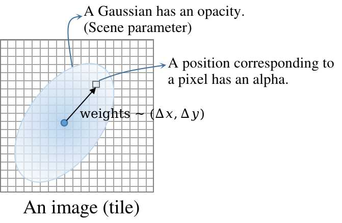
$$ \underset{\substack{↑\\ \text{Pixel}\\ \text{color}}}{C} = ∑_{k∈N} \underset{\substack{↑\\ \text{Kernel}\\ \text{weight}}}{wₖ}⋅ \underset{\substack{↑\\ \text{Kernel} \\ \text{color}}}{cₖ}⋅ \underset{\substack{↑\\ \text{Accumulated} \\ \text{transmittance}}}{oₖ}⋅ (\underset{\substack{↑\\ \text{Kernel}\\ \text{opacity}}}{qₖ}⊗ \underset{\substack{↑\\ \text{Loss-pass}\\ \text{filter}}}{h}) (\underset{\substack{↑\\ \text{2D} \\ \text{coords}}}{𝐱}) $$

In 3DGS, each 3D Gassian in the object space has 4 learnable parameters:

1. Color (cₖ): SH for “directional appearance component of the radiance field”

2. Opacity ($qₖ⊗ h$). It results in accu. transmittance oₖ as $∏_{m≤k}(1-\text{opacity}ₘ)$.

3. Position 𝛍: determines the kernel’s weight wₖ, as wₖ is an evaluation of the projected kernel (2D Gaussian distribution) at the pixel.

4. Covariance matrix: the stretching matrix and rotaion matrix (quaternion) jointly determine wₖ as well.

The splatting equation can be reformulated as alpha compositing used in 3DGS:

$$C = ∑_{n≤N} Tₙ⋅αₙ⋅cₙ, \text{ where } Tₙ = ∏_{m≤n}(1-αₘ)$$

• Alpha can be expressed with sigma, which is an exponent of e, akin to NeRF.

  $$αₙ = oₙ ⋅ exp(-σₙ), \text{where } σₙ = ½\bm Δₙᵀ \bm Σ’⁻¹ \bm Δₙ$$

  • oₙ is a kernel’s opacity, i.e., the above qₖ⊗ h. And the negative exponential term is a scalar scaling factor. σₙ is Mahalanobis distance.

    (2024-02-16)

    • Gaussian’s opacity oₙ is fixed after splatting with a specific viewing ray, so during alpha compositing, the variation in alpha among different Gaussian results from the different positions of a target rendering pixel relative to various Gaussians.

      When performing alpha compositing, the alpha of a Gaussian is the Gaussian’s opacity scaled by the “probability” for the position of the rendering pixel in the Gaussian distribution.

  • However, the alpha value in NeRF is $αᵢ = 1- exp(-σᵢδᵢ)$ and serves as the opacity in $∑ᵢ₌₁ᴺ Tᵢ αᵢ cᵢ$. Alpha is a converted point opacity ranging in [0,1].

• In other words, alpha $αₙ$ equals a kernel’s opacity oₙ scaled by a weight Gₙ (the above wₖ), i.e., the evaluation of 2D Gaussian Gₙ at the viewing pixel:

  $$αₙ = oₙ ⋅ Gₙ, \text{where } Gₙ = e^{-\frac{\bm Δₙᵀ \bm Δₙ}{2\bm Σ’}}$$

  • oₙ is the opacity (the footprint qₙ) of the n-th 3D Gaussian. qₙ is an integral of the Gaussian in the 3D ray space along the viewing ray: $qₙ(𝐱) = ∫rₙ’(𝐱,x₂)dx₂$.

  • oₙ will get optimized directly via gradient descent during training.

  • Gₙ is a 2D Gaussian with the normalization factor omitted. Its mean and covariance matrix will get optimized.

  • Δₙ is the displacement of a pixel center from the 2D Gaussian’s mean.

    

• Initially, the opacity of an arbitrary 3D location in the object space is considered as an expectation of the contributions from all 3D Gaussians on that location.

  After ❶ substituting the perspectively projected (“squashed”) kernel within the 3D ray space into the rendering equation, ❷ switching the sequence of integral and expectation, ❸ and applying simplifying assumptions, the opacity becomes a 1-D (depth) integral along the viewing ray for each kernel in the 3D ray space.

  In summary, the changes of opacity before and after perspective projection:

  Aspect	Original form	Post-projection
  Venue	Object space	3D ray space, or screen
  Intuition	Opacity combination	Discs stack
  Scope	Location-wise	Ellipsoid-wise
  Operation	Expectation	Integral
  Formula	$f_c(𝐮) = ∑_{k≤N} wₖ rₖ(𝐮)$	Footprint $qₖ(𝐱) = ∫_{x₂=0}^L rₖ’(𝐱,x₂) dx₂$
  Basis	Gauss. mixture	Scene locality

  • Locality: 3D positions are grouped into different ellipsoids.

• (2024-01-06) A 3D Gaussian (datapoint) in the camera space (or clip space) is “perspectively” projected (thrown) onto the screen (or the ray space, as its x2 is independtly assigned beside the screen coordinates x0,x1), and results in a 2D Gaussian (with applying the Taylor expansion to approximate the nonlinear perspective effects).

  The viewing ray in camera space will be projected into the 3D ray space remaining a straight line segment (due to the linear approximation), and then the 3D line is projected onto the screen orthogonally.

  Orthogonal projection is because the 3D Gaussians have already been projected onto the screen (the location has been determined as x,y divided by z and covariance matrix 𝚺’= 𝐉𝐖 𝚺𝐖ᵀ 𝐉ᵀ) yielding 2D Gaussians, so each pixel is only derived from those projected kernels (2D Gaussians) that overlaps with it (“Overlapping” refer to 3DGS.), like a stack of filters in alpha compositing. That implies the alpha compositing is performed in the screen space, or the ray sapce, as the ray space is equivalent with screen (EWA paper: “the transformation from volume-data to ray space is equivalent to perspective projection.”).

  With the “orthogonal correspondence” between the ray space and the screen, the ray integral (footprint function, or kernel’s opacity) in the 3D ray space becomes (??Not sure) an integral on the 2D screen plane, i.e., an integral of a 2D Gaussian.

  And the ray in the 3D ray space corresponds to a line on the screen, as rays in the 3D ray space are parallel (i.e., orthogonal projection). Thus, the opacity is an

Alpha of an arbitrary point in screen (or 3D ray space) is a 2D-Gaussian mixture over all kernels. (Not the screen, object space is opacities combination, whereas the screen space is filter stacking.)

The alpha of a 3D location is calculated in each 3D Gaussian based on the distance to the center. And the final alpha on the location is the expectation of all the evaluations. (No location-wise alpha was calculated.)

The color of a pixel on the screen is a 2D-Gaussian mixture:

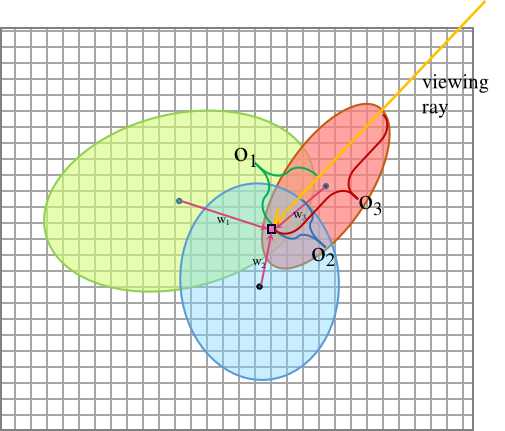
The alpha compositing process for a pixel is illustrated below:

• Opacities (o₁,o₂,o₃) of different kernels are various-length integral along the viewing ray in the 3D ray space.

  • Not sure whether the integral in 3D ray space equal the integral on screen.

• Weight (w₁,w₂,w₃) of a kernel’s opacity is its evaluation at the pixel.

• Alpha (α₁,α₂,α₃) of a kernel equals its opacity multiplied with its weight.

• Accumulated transmittance (T₁,T₂,T₃) equals the product of previously passed kernels’ transmittance.

• Pixel color is the sum of each kernel’s color scaled by alpha.

There is no volume rendering as there is no sampling points on the viewing ray. Pixel is a summation of visible 2D discs (referring to 3DGS). Only alphas of the explicitly existent discs require to be computed, unlike volume rendering where every sampling location need to compute alpha.

Gradient wrt Composite

(2023-01-07)

• The dot lines in the left figure represent orthogonal correspondence, not projection.
• A pixel can only see 2D Gaussians located on its perpendicular line.
• Those visible 2D Gaussians to a pixel are sorted based on depth, and then their colors are composited from near to far with multiplying with their opacities that computed as an integral along the viewing ray.

A synthesized pixel is a weighted sum of the related (overlapping) kernels’ color in the whole space:

$$C_{pred} = ∑_{n≤N} Tₙ⋅αₙ⋅cₙ, \quad \text{where } αₙ=oₙ⋅e^{-\frac{\bm Δₙᵀ \bm Δₙ}{2\bm Σ’}}$$

Loss:

$$L = ‖C_{targ} - C_{pred}‖₂$$

1
2
3

fc = nn.Linear(3, 10)   # fc.weight is (10,3)
x = torch.range(2,3)
fc(x)   # X⋅Wᵀ = (2,3)⋅(3,10) = (2,10) is ⟨Xᵀ,Wᵀ⟩

Since the passed kernels on the ray path (starting from a pixel) have influences on the next kernel’s contribution, which is scaled by the previous accumulated transmittance, the order of solving derivatives should start from the most rear kernel, and then sequentially calculate the derivatives of front kernels in the reverse order of the forward pass.

• The viewing ray travels from back to front and hits the screen. But the color nearest to the screen is the first to be seen by (or shown on) the camera (or eye).

• The toppest color is based on downstream colors, so, its a function of all the preceding colors.

  In the color stack, the color above depends on color below. Thus, the derivatives at the bottom should be sovled first.

  (2024-01-16) The toppest color is the base of all downstream colors, so, its derivative is contributed by all the behind colors.

Color, Opacity

(2024-01-08)

Given $\frac{∂L}{∂Cᵢ(k)}$, the partial derivatives of the predicting pixel color $Cᵢ$ w.r.t. each parameter of a Gaussian Gₙ (in the ray space) that contributes to the pixel are:

1. The parital derivative of Cᵢ w.r.t. the kernel Gₙ’s color cₙ, based on the forward pass: $Cᵢ = T₁⋅α₁⋅c₁+ T₂⋅α₂⋅c₂ + ⋯ Tₙ⋅αₙ⋅cₙ+ Tₙ₊₁⋅αₙ₊₁⋅cₙ₊₁ +⋯ + T_N⋅α_N⋅c_N$:

   $$\frac{∂Cᵢ(k)}{∂cₙ(k)} = αₙ⋅Tₙ$$

   • k represents one channel of RGB.

   • The furthest $T_N$ from the screen is saved at the end of the forward pass. And then the $T_{N-1}$ in front of it is calculated as $T_{N-1} = \frac{T_N}{1-α_{N-1}}$. The points in front follow this relation.

   3DGS Code

   1 2	T = T / (1.f - alpha); const float dchannel_dcolor = alpha * T;

2. Alpha αₙ

   To solve the partial derivative of pixel color $C_i$ w.r.t. the kernel Gₙ’s αₙ, only consider the kernels that follow Gₙ, as the transmittances of all the subsequent kernels rely on the currenct kernel Gₙ: $$Tₙ₊₁ = (1-αₙ)Tₙ$$

   Thereby, the behind kernels will provide derivatives to the current kernel Gₙ’s alpha.

   For example, the color of the next kernel, Gₙ₊₁, behind Gₙ is:

   $$\begin{aligned} Cₙ₊₁ &= cₙ₊₁⋅αₙ₊₁⋅Tₙ₊₁ \\ &= cₙ₊₁⋅αₙ₊₁⋅ (1-αₙ)Tₙ \\ &= cₙ₊₁⋅αₙ₊₁⋅(1-αₙ)⋅ \frac{ Tₙ₊₁}{1-αₙ} \\ \end{aligned}$$

   Thus, the color $Cₙ₊₁$ contributes to the total partial derivative $\frac{∂Cᵢ}{∂αₙ}$ with the amount: $-\frac{cₙ₊₁⋅αₙ₊₁⋅Tₙ₊₁}{1-αₙ}$ .

   Continuously, the following color Cₙ₊₂ can be represented with αₙ:

   $$ Cₙ₊₂ = cₙ₊₂⋅αₙ₊₂⋅Tₙ₊₂ \\ = cₙ₊₂⋅αₙ₊₂ ⋅\cancel{(1-αₙ₊₁)} (1-αₙ) \frac{Tₙ₊₂}{ \cancel{(1-αₙ₊₁)} (1-αₙ)}$$

   • Thus, $\frac{∂Cₙ₊₂}{∂αₙ} = -\frac{cₙ₊₂⋅αₙ₊₂⋅Tₙ₊₂}{1-αₙ}$

   Similarly, the subsequent kernel Gₘ, with m>n, also contribute to the overall partial derivative $\frac{∂Cᵢ}{∂αₙ}$.

   Thereby, the ultimate partial derivatives of the pixel color $Cᵢ$ w.r.t. the Gₙ’s alpha αₙ is:

   $$\frac{∂Cᵢ}{∂αₙ} = cₙ⋅Tₙ - \frac{∑_{m>n}cₘ⋅αₘ⋅ Tₘ}{1-αₙ}$$

3. Opacity oₙ, mean 𝛍’, and covariance 𝚺':

   According to $αₙ = oₙ e^{-σₙ}$, where $σₙ = \frac{\bm Δₙᵀ \bm Δₙ}{2\bm Σₙ’}$ (a scalar), and 𝚫ₙ is the offset from the pixel center to the 2D Gaussian Gₙ’s mean $\bm μ’$, such as $\bm Δₙ = \bm μₙ’ - 𝐱ᵢ$.

   • Partial derivative of αₙ w.r.t. opacity oₙ:

     $$ \frac{∂αₙ}{∂oₙ} = e^{-\frac{\bm Δₙᵀ \bm Δₙ}{2\bm Σₙ’}} $$

   • Partial derivative of αₙ w.r.t. the “exponent” sigma $σₙ$:

     $$ \frac{∂αₙ}{∂σₙ} = -oₙ e^{-σₙ}$$

   • Partial derivative of sigma σₙ w.r.t. 2D mean 𝛍ₙ':

     Because $\bm Δₙ$ is a function of 𝛍ₙ’, computing derivaties w.r.t. 𝛍ₙ’ is equivalent to $\bm Δₙ$.

     The Jacobian of σₙ is:

     $$\frac{∂σₙ}{∂\bm μₙ’} = \frac{∂σₙ}{∂\bm Δₙ’} = \frac{∂(½\bm Δₙ’ᵀ \bm Σ’⁻¹ \bm Δₙ’)}{∂\bm Δₙ’} = \bm Σₙ’⁻¹ \bm Δₙ’$$

   • Partial derivative of sigma σₙ w.r.t. 2D covariance matrix 𝚺':

     $$\frac{∂σₙ}{∂\bm Σₙ’} =$$

Gradient wrt Projection

(2024-01-10)

A 3D Gaussian distribution centered at 𝛍ₖ with a covariance matrix 𝚺ₖ in the object space will be projected onto 2D screen through the splatting step, resulting in a 2D Gaussian distribution, with applying the affine transformation approximation for the nonlinear perspective division.

The 3D ray space (or the screen) is constructed based on the perspective division (x,y divided by z), which however is non-linear. Therefore, the projective transformation $ϕ(𝐭’)$ (i.e., perspective division + new depth) converting the clip space to the 3D ray space is approximated by a linear mapping: $ϕₖ(𝐭’) = ϕ(𝐭ₖ’) + 𝐉ₖ⋅(𝐭’ - 𝐭ₖ’)$, where 𝐭ₖ’ = 𝛍ₖᶜ, the mean vector in clip space.

The effects of the approximated affine mapping ϕₖ(𝐭’) are as follows:

1. The transformed 2D Gaussian’s center 𝛍ₖ’ is the exact projective transformation ϕ(𝛍ₖᶜ), i.e., ϕₖ(𝐭ₖ’)=ϕ(𝐭ₖ’), without any error, with the 3rd dimension omitted.

   $$ \underset{(3D)}{\bm μₖ’} = ϕ(\bm μₖᶜ) = \begin{bmatrix} f_x⋅μ_{k,x}ᶜ/μ_{k,z}ᶜ + c_x \\ f_y⋅μ_{k,y}ᶜ/μ_{k,z}ᶜ + c_y \\ \sqrt{ {μ_{k,x}ᶜ}^2 + {μ_{k,y}ᶜ}^2 + {μ_{k,z}ᶜ}^2} \end{bmatrix} \overset{\text{Omit 3rd dim}}{\longrightarrow} \underset{(2D)}{\bm μₖ’}= \begin{bmatrix} \frac{f_x⋅μ_{k,x}ᶜ}{μ_{k,z}ᶜ} + c_x \\ \frac{f_y⋅μ_{k,y}ᶜ}{μ_{k,z}ᶜ} + c_y \end{bmatrix} $$

2. However, the approximated transformation ϕₖ(𝐭’) of an arbitrary point 𝐭’ around the clip-space 3D Gaussian center 𝐭ₖ' will deviate from the precise perspective projections ϕ(𝐭’) gradually, as the (𝐭’ - 𝐭ₖ’) increases in the approximated mapping:

   $$ \begin{aligned} ϕ(𝐭’) ≈ ϕₖ(𝐭’) &= ϕ(𝐭ₖ’) + 𝐉ₖ⋅(𝐭’ - 𝐭ₖ’) \\ &= \bm μₖ’ + 𝐉ₖ⋅(𝐭’ - 𝐭ₖ’) \end{aligned} $$

3. The projected 2x2 covariance matrix on screen is the 3x3 matrix in the ray space: $\bm Σₖ’ = 𝐉ₖ⋅ 𝐑_{w2c}⋅ \bm Σₖ⋅ 𝐑_{w2c}ᵀ⋅ 𝐉ₖᵀ$, with the 3rd row and column omitted.

(2024-01-11)

⭐Note: The following $𝐭ₖ$ is the coordinates of a Gaussian center in the camera space: $$𝐭ₖ = [^{𝐑_{w2c} \ 𝐭_{w2c}}_{0 \quad\ 1}] ⋅[^{\bm μₖ}_1]$$

• where 𝛍ₖ³ᕽ¹ is the coordinates of the mean vector in world space.

• $𝐭’$ is the clip coordinates, which is camera coordinates times the projection matrix 𝐏: $𝐭’ = 𝐏𝐭$

• 𝐏 maps the camera-space coordinates to camera film (homogeneous) and scales for letting the ND Coordinates of points located within the camera frustum range in [-1,1]. With using clip coordinates, points whose w (i.e., z) is smaller than x,y,z are deleted.

• The approximated projective transformation $ϕₖ(𝐭’)$ fulfills perspective division after frustum clipping. Therefore, the 2D screen coordinates $\bm μₖ’_{(2D)} = ϕₖ(𝐭ₖ’)_{(2D)}$ are NDC ∈ [-1,1].

• Then the Gaussian center’s ND coordinates are scaled back to the screen size, yielding pixel coordinates 𝛍ₖ’₍ₚᵢₓ₎ represented with clip coordinates as:

  $$ \bm μₖ’_{(\text{pix})} = \begin{bmatrix} (W⋅t_{k,x}’/t_{k,w}’ + 1) /2 + c_x \\ (H⋅t_{k,y}’/t_{k,w}’ + 1) / 2 + c_y \end{bmatrix} $$

  This relationship enables propagating gradients from pixel coordinates $\bm μₖ’₍ₚᵢₓ₎$ to the clip coordinates $𝐭ₖ’$ directly, without the 2D screen coordinates $\bm μₖ’_{(2D)}$ involved.

Center

(2024-01-12)

Because 𝛍ₖ’₍ₚᵢₓ₎ and 𝚺ₖ’ on the 2D screen both are functions of 3D Gaussian center 𝐭ₖ, the partial derivatives of the loss w.r.t. 𝐭ₖ³ᕽ¹ is a sum:

$$ \frac{∂L}{∂𝐭ₖ} = \frac{∂L}{∂ \bm μₖ’₍ₚᵢₓ₎} \frac{∂\bm μₖ’₍ₚᵢₓ₎}{∂𝐭ₖ} + \frac{∂L}{∂\bm Σₖ’_{(2D)}} \frac{∂\bm Σₖ’_{(2D)}}{∂𝐭ₖ} \\ $$

1. The partial derivative of 2D Gaussian’s mean $\bm μₖ’₍ₚᵢₓ₎$ w.r.t. the camera coordinates of 3D Gaussian center 𝐭ₖ:

   $$ \begin{aligned} \frac{∂\bm μₖ’₍ₚᵢₓ₎}{∂𝐭ₖ} &= \frac{∂\bm μₖ’₍ₚᵢₓ₎}{∂\bm μₖ’_{(2D)}} ⋅ \frac{∂ϕₖ(𝐭ₖ’)_{(2D)}}{𝐭ₖ’} ⋅ \frac{∂𝐭ₖ’}{∂𝐭ₖ} \qquad \text{(Full process)} \\ &= \frac{∂\bm μₖ’₍ₚᵢₓ₎}{∂𝐭ₖ’} ⋅ \frac{∂𝐭ₖ’}{∂𝐭ₖ} \qquad \text{(Clip→Pix, skip screen coords)} \\ &= \frac{1}{2} \begin{bmatrix} W/t_{k,w}’ & 0 & 0 & -W⋅t_{k,x}’/{t_{k,w}’}^2 \\ 0 & H/t_{k,w}’ & 0 & -H⋅t_{k,y}’/{t_{k,w}’}^2 \end{bmatrix}⋅ 𝐏 \end{aligned} $$

   Based on the properties of the Frobenius inner product, eq. (23) is obtained.

2. The partial derivative of the 2D Gaussian’s covariance 𝚺ₖ’ w.r.t. the camera coordinates of 3D Gaussian center 𝐭ₖ:

   $$ \frac{∂\bm Σₖ’}{∂𝐭ₖ} = \frac{∂(𝐉ₖ⋅ 𝐑_{w2c}⋅ \bm Σₖ⋅ 𝐑_{w2c}ᵀ⋅ 𝐉ₖᵀ)_{2D} }{∂𝐭ₖ} $$

   (2024-01-13) Derivation refers to 3D Gaussian Splatting中的数学推导 - 八氨合氯化钙的文章 - 知乎

   1. Letting $𝐔 = 𝐉ₖ⋅ 𝐑_{w2c}$ (3DGS code refers to it as T.), the Gaussian covariance 𝚺ₖ’ in the 3D ray space derived from the projective transformation ϕₖ(𝐭’) is:

      $$\bm Σₖ’ = 𝐔 ⋅ \bm Σₖ⋅𝐔ᵀ = \\ \begin{bmatrix} U₁₁ & U₁₂ & U₁₃ \\ U₂₁ & U₂₂ & U₂₃ \\ U₃₁ & U₃₂ & U₃₃ \end{bmatrix} \begin{bmatrix} σ₁₁ & σ₁₂ & σ₁₃ \\ σ₂₁ & σ₂₂ & σ₂₃ \\ σ₃₁ & σ₃₂ & σ₃₃ \end{bmatrix} \begin{bmatrix} U₁₁ & U₂₁ & U₃₁ \\ U₁₂ & U₂₂ & U₃₂ \\ U₁₃ & U₂₃ & U₃₃ \end{bmatrix} = \\ \begin{bmatrix} U₁₁ & U₁₂ & U₁₃ \\ U₂₁ & U₂₂ & U₂₃ \\ U₃₁ & U₃₂ & U₃₃ \end{bmatrix} \begin{bmatrix} \boxed{σ₁₁}U₁₁+σ₁₂U₁₂+σ₁₃U₁₃ & \boxed{σ₁₁}U₂₁+σ₁₂U₂₂+σ₁₃U₂₃ & \boxed{σ₁₁}U₃₁+σ₁₂U₃₂+σ₁₃U₃₃ \\ σ₂₁U₁₁+σ₂₂U₁₂+σ₂₃U₁₃ & σ₂₁U₂₁+σ₂₂U₂₂+σ₂₃U₂₃ & σ₂₁U₃₁+σ₂₂U₃₂+σ₂₃U₃₃ \\ σ₃₁U₁₁+σ₃₂U₁₂+σ₃₃U₁₃ & σ₃₁U₂₁+σ₃₂U₂₂+σ₃₃U₂₃ & σ₃₁U₃₁+σ₃₂U₃₂+σ₃₃U₃₃ \end{bmatrix} = \\ \Big[ \begin{array}{c|c|c} U₁₁(σ₁₁U₁₁+σ₁₂U₁₂+σ₁₃U₁₃) + U₁₂(σ₂₁U₁₁+σ₂₂U₁₂+σ₂₃U₁₃) + U₁₃(σ₃₁U₁₁+σ₃₂U₁₂+σ₃₃U₁₃) & U₁₁(σ₁₁U₂₁+σ₁₂U₂₂+σ₁₃U₂₃) + U₁₂(σ₂₁U₂₁+σ₂₂U₂₂+σ₂₃U₂₃) + U₁₃(σ₃₁U₂₁+σ₃₂U₂₂+σ₃₃U₂₃) & U₁₁(σ₁₁U₃₁+σ₁₂U₃₂+σ₁₃U₃₃) + U₁₂(σ₂₁U₃₁+σ₂₂U₃₂+σ₂₃U₃₃) + U₁₃(σ₃₁U₃₁+σ₃₂U₃₂+σ₃₃U₃₃) \\ U₂₁(σ₁₁U₁₁+σ₁₂U₁₂+σ₁₃U₁₃) + U₂₂(σ₂₁U₁₁+σ₂₂U₁₂+σ₂₃U₁₃) + U₂₃(σ₃₁U₁₁+σ₃₂U₁₂+σ₃₃U₁₃) & U₂₁(σ₁₁U₂₁+σ₁₂U₂₂+σ₁₃U₂₃) + U₂₂(σ₂₁U₂₁+σ₂₂U₂₂+σ₂₃U₂₃) + U₂₃(σ₃₁U₂₁+σ₃₂U₂₂+σ₃₃U₂₃) & U₂₁(σ₁₁U₃₁+σ₁₂U₃₂+σ₁₃U₃₃) + U₂₂(σ₂₁U₃₁+σ₂₂U₃₂+σ₂₃U₃₃) + U₂₃(σ₃₁U₃₁+σ₃₂U₃₂+σ₃₃U₃₃) \\ U₃₁(σ₁₁U₁₁+σ₁₂U₁₂+σ₁₃U₁₃) + U₃₂(σ₂₁U₁₁+σ₂₂U₁₂+σ₂₃U₁₃) + U₃₃(σ₃₁U₁₁+σ₃₂U₁₂+σ₃₃U₁₃) & U₃₁(σ₁₁U₂₁+σ₁₂U₂₂+σ₁₃U₂₃) + U₃₂(σ₂₁U₂₁+σ₂₂U₂₂+σ₂₃U₂₃) + U₃₃(σ₃₁U₂₁+σ₃₂U₂₂+σ₃₃U₂₃) & U₃₁(σ₁₁U₃₁+σ₁₂U₃₂+σ₁₃U₃₃) + U₃₂(σ₂₁U₃₁+σ₂₂U₃₂+σ₂₃U₃₃) + U₃₃(σ₃₁U₃₁+σ₃₂U₃₂+σ₃₃U₃₃) \end{array} \Big] $$

      The 3rd row and column in 𝚺ₖ’ are omitted due to the orthogonal correspondence between the 3D ray space and the 2D screen. Thus, $\bm Σₖ’_{(2D)}$ is only the upper-left 2×2 elements of the 3D 𝚺ₖ’, contributing to the gradient of 2D loss $L(𝐜ₖ, oₖ, \bm μₖ’_{(2D)}, \bm Σₖ’_{(2D)})$, while the remaining 5 elements of 𝚺ₖ’₍₃ₓ₃₎ make no contributions.

      $$ \bm Σₖ’_{(2D)} = \\ \Big[ \begin{array}{c|c} U₁₁(σ₁₁U₁₁+σ₁₂U₁₂+σ₁₃U₁₃) + U₁₂(σ₂₁U₁₁+σ₂₂U₁₂+σ₂₃U₁₃) + U₁₃(σ₃₁U₁₁+σ₃₂U₁₂+σ₃₃U₁₃) & U₁₁(σ₁₁U₂₁+σ₁₂U₂₂+σ₁₃U₂₃) + U₁₂(σ₂₁U₂₁+σ₂₂U₂₂+σ₂₃U₂₃) + U₁₃(σ₃₁U₂₁+σ₃₂U₂₂+σ₃₃U₂₃) \\ U₂₁(σ₁₁U₁₁+σ₁₂U₁₂+σ₁₃U₁₃) + U₂₂(σ₂₁U₁₁+σ₂₂U₁₂+σ₂₃U₁₃) + U₂₃(σ₃₁U₁₁+σ₃₂U₁₂+σ₃₃U₁₃) & U₂₁(σ₁₁U₂₁+σ₁₂U₂₂+σ₁₃U₂₃) + U₂₂(σ₂₁U₂₁+σ₂₂U₂₂+σ₂₃U₂₃) + U₂₃(σ₃₁U₂₁+σ₃₂U₂₂+σ₃₃U₂₃) \end{array} \Big] $$

      • Each element of $\bm Σₖ’_{(2D)}$ is a “sub-” function, which is taken derivative w.r.t. each variable: σ₁₁, σ₁₂, σ₁₃, σ₂₂, σ₂₃, σ₃₃, to backpropagate the gradient $\frac{∂L}{∂\bm Σₖ’_{(2D)}}$ to 𝚺ₖ. (Only these 6 elements of 𝚺ₖ need computation as 𝚺ₖ₍₃ₓ₃₎ is symmetric.)

      • It’s not proper to think of the derivative of a “matrix” w.r.t. a matrix. Instead, it’s better to consider the derivative of a function w.r.t. variables, as essentially a matrix stands for a linear transformation.

      The partial derivative of $\bm Σₖ’_{(2D)}$ w.r.t. $\bm Σₖ$ (the 3D covariance matrix in world space):

      $$ \frac{∂\bm Σₖ’_{(2D)}}{∂σ₁₁} = \begin{bmatrix} U₁₁U₁₁ & U₁₁U₂₁ \\ U₂₁U₁₁ & U₂₁U₂₁ \end{bmatrix} = \begin{bmatrix} U₁₁ \\ U₂₁ \end{bmatrix} \begin{bmatrix} U₁₁ & U₂₁ \end{bmatrix} \\ \frac{∂\bm Σₖ’_{(2D)}}{∂σ₁₂} = \begin{bmatrix} U₁₁U₁₂ & U₁₁U₂₂ \\ U₂₁U₁₂ & U₂₁U₂₂ \end{bmatrix} = \begin{bmatrix} U₁₁ \\ U₂₁ \end{bmatrix} \begin{bmatrix} U₁₂ & U₂₂ \end{bmatrix} \\ \frac{∂\bm Σₖ’_{(2D)}}{∂σ₁₃} = \begin{bmatrix} U₁₁U₁₃ & U₁₁U₂₃ \\ U₂₁U₁₃ & U₂₁U₂₃ \end{bmatrix} = \begin{bmatrix} U₁₁ \\ U₂₁ \end{bmatrix} \begin{bmatrix} U₁₃ & U₂₃ \end{bmatrix} \\ \frac{∂\bm Σₖ’_{(2D)}}{∂σ₂₂} = \begin{bmatrix} U₁₂U₁₂ & U₁₂U₂₂ \\ U₂₂U₁₂ & U₂₂U₂₂ \end{bmatrix} = \begin{bmatrix} U₁₂ \\ U₂₂ \end{bmatrix} \begin{bmatrix} U₁₂ & U₂₂ \end{bmatrix} \\ \frac{∂\bm Σₖ’_{(2D)}}{∂σ₂₃} = \begin{bmatrix} U₁₂U₁₃ & U₁₂U₂₃ \\ U₂₂U₁₃ & U₂₂U₂₃ \end{bmatrix} = \begin{bmatrix} U₁₂ \\ U₂₂ \end{bmatrix} \begin{bmatrix} U₁₃ & U₂₃ \end{bmatrix} \\ \frac{∂\bm Σₖ’_{(2D)}}{∂σ₃₃} = \begin{bmatrix} U₁₃U₁₃ & U₁₃U₂₃ \\ U₂₃U₁₃ & U₂₃U₂₃ \end{bmatrix} = \begin{bmatrix} U₁₃ \\ U₂₃ \end{bmatrix} \begin{bmatrix} U₁₃ & U₂₃ \end{bmatrix} $$

      • σ₁₁, σ₂₂, σ₃₃ are on the diagonal, while σ₁₂, σ₁₃, σ₂₃ are off-diagonal.

      The partial derivative of the loss L w.r.t. each element of 𝚺ₖ:

      $$ \begin{aligned} \frac{∂L}{∂\bm Σₖ’_{(2D)}} \frac{∂\bm Σₖ’_{(2D)}}{∂σ₁₁} &= ∑_{row}∑_{col}{ \begin{bmatrix} \frac{∂L}{∂a} & \frac{∂L}{∂b} \\ \frac{∂L}{∂b} & \frac{∂L}{∂c} \end{bmatrix} ⊙ \begin{bmatrix} U₁₁U₁₁ & U₁₁U₂₁ \\ U₂₁U₁₁ & U₂₁U₂₁ \end{bmatrix} } \\ &= \frac{∂L}{∂a} U₁₁U₁₁ + 2× \frac{∂L}{∂b} U₁₁U₂₁ + \frac{∂L}{∂c} U₂₁U₂₁ \\ \frac{∂L}{∂\bm Σₖ’_{(2D)}} \frac{∂\bm Σₖ’_{(2D)}}{∂σ₁₂} &= ∑_{row}∑_{col}{ \begin{bmatrix} \frac{∂L}{∂a} & \frac{∂L}{∂b} \\ \frac{∂L}{∂b} & \frac{∂L}{∂c} \end{bmatrix} ⊙ \begin{bmatrix} U₁₁U₁₂ & U₁₁U₂₂ \\ U₂₁U₁₂ & U₂₁U₂₂ \end{bmatrix} } \\ &= \frac{∂L}{∂a} U₁₁U₁₂ + \frac{∂L}{∂b} U₁₁U₂₂ +\frac{∂L}{∂b}U₂₁U₁₂ + \frac{∂L}{∂c} U₂₁U₂₂ \end{aligned} $$

      • ⊙ is Hadamard product (element-wise product). $∑_{row}∑_{col}$ means summation of all elements in the matrix.

        (2024-02-17) In this step, the derivative w.r.t. a matrix is determined by calculating the derivative w.r.t. each element individually, rather than the entire matrix. Thus, the multiplication between two “derivative matrices” is hadamard product, as essentially it’s the derivative w.r.t. a single scalar (in contrast to vector or matrix). However, for example, if $\frac{∂\bm Σ}{∂𝐌}$ is the derivative of 𝚺 w.r.t. the matrix 𝐌, the multiplication with the incoming upstream “derivative matrix” should be a normal matmul.

        Within a chain of differentiation, the 2 manners of solving derivative for a matrix by computing the derivative for the entire matrix or calculating the derivative for each element can coexist simultaneously.

      • Note: The $\frac{∂L}{∂b}$ in the 3DGS code has been doubled. And each off-diagonal element is multiplied by 2, as the symmetrical element has the same gradient contribution.

      In 3DGS code, the derivative of loss w.r.t. each element of 3D covariance matrix 𝚺ₖ₍₃ₓ₃₎ in the world space is computed individually:

      1 2 3 4 5 6 7 8 9 10 11

      dL_da = denom2inv * (...); dL_dc = denom2inv * (...); dL_db = denom2inv * 2 * (...); dL_dcov[0] = (T[0][0]*T[0][0]*dL_da + T[0][0]*T[1][0]*dL_db + T[1][0]*T[1][0]*dL_dc); dL_dcov[3] = (T[0][1]*T[0][1]*dL_da + T[0][1]*T[1][1]*dL_db + T[1][1]*T[1][1]*dL_dc); dL_dcov[5] = (T[0][2]*T[0][2]*dL_da + T[0][2]*T[1][2]*dL_db + T[1][2]*T[1][2]*dL_dc); dL_dcov[1] = 2*T[0][0]*T[0][1]*dL_da + (T[0][0]*T[1][1] + T[0][1]*T[1][0])*dL_db + 2*T[1][0]*T[1][1]*dL_dc; dL_dcov[2] = 2*T[0][0]*T[0][2]*dL_da + (T[0][0]*T[1][2] + T[0][2]*T[1][0])*dL_db + 2*T[1][0]*T[1][2]*dL_dc; dL_dcov[4] = 2*T[0][2]*T[0][1]*dL_da + (T[0][1]*T[1][2] + T[0][2]*T[1][1])*dL_db + 2*T[1][1]*T[1][2]*dL_dc;

      The 2D covariance matrix $\bm Σₖ’_{(2D)}$ is Not equivalent to the calculation where the 3rd row and column of 𝚺ₖ are omitted from the beginning, because σ₁₃, σ₂₃, σ₃₃ are also involved in the projected covariance 𝚺ₖ’. However, the derivatives w.r.t. them ($\frac{∂\bm Σₖ’_{(2D)}}{∂σ₁₃},\ \frac{∂\bm Σₖ’_{(2D)}}{∂σ₂₃},\ \frac{∂\bm Σₖ’_{(2D)}}{∂σ₃₃}$) can’t be derived from the following expression:

      $$\begin{aligned} \bm Σₖ’_{(2D)} &= \begin{bmatrix} U₁₁ & U₁₂ \\ U₂₁ & U₂₂ \end{bmatrix} \begin{bmatrix} σ₁₁ & σ₁₂ \\ σ₂₁ & σ₂₂ \end{bmatrix} \begin{bmatrix} U₁₁ & U₂₁ \\ U₁₂& U₂₂ \end{bmatrix} \\ &= \begin{bmatrix} (U₁₁σ₁₁ + U₁₂σ₂₁)U₁₁ + (U₁₁σ₁₂ + U₁₂σ₂₂) U₁₂ & (U₁₁σ₁₁ + U₁₂σ₂₁)U₂₁ + (U₁₁σ₁₂ + U₁₂σ₂₂) U₂₂ \\ (U₂₁σ₁₁ + U₂₂σ₂₁)U₁₁ + (U₂₁σ₁₂ + U₂₂σ₂₂) U₁₂ & (U₂₁σ₁₁ + U₂₂σ₂₁)U₂₁ + (U₂₁σ₁₂ + U₂₂σ₂₂) U₂₂ \end{bmatrix} \end{aligned} $$

   2. The partial derivative of the 2D Gaussian covariance matrix $\bm Σₖ’_{(2D)}$ w.r.t. the 3D Gaussian center 𝐭ₖ in the camera space:

      $$ \begin{aligned} \frac{∂\bm Σₖ’_{(2D)}}{∂𝐔ₖ} \frac{∂𝐔ₖ}{∂𝐭ₖ} = \frac{∂𝐔ₖ {\bm Σₖ}_{(3D)} 𝐔ₖᵀ}{∂𝐔ₖ} \frac{∂(𝐉ₖ⋅ 𝐑_{w2c})}{∂𝐭ₖ} \\ \end{aligned} $$

      • $\frac{∂𝐔ₖ {\bm Σₖ}_{(3D)} 𝐔ₖᵀ}{∂𝐔ₖ}$ (corresponding to $\frac{∂\bm Σₖ’}{∂T}$ inside $\frac{∂L}{∂T}$ of eq.(25) in the gsplat paper.)

        $$ \begin{aligned} \frac{∂𝐔ₖ {\bm Σₖ}_{(3D)} 𝐔ₖᵀ}{∂U₁₁} &= \begin{bmatrix} 2σ₁₁U₁₁+(σ₁₂+σ₂₁)U₁₂+(σ₁₃+σ₃₁)U₁₃ & σ₁₁U₂₁+σ₁₂U₂₂+σ₁₃U₂₃ & σ₁₁U₃₁+σ₁₂U₃₂+σ₁₃U₃₃ \\ σ₁₁U₂₁ + σ₂₁U₂₂ + σ₃₁U₂₃ & 0 & 0 \\ σ₁₁U₃₁ + σ₂₁U₃₂ + σ₃₁U₃₃ & 0 & 0 \end{bmatrix} \\ \frac{∂𝐔ₖ {\bm Σₖ}_{(3D)} 𝐔ₖᵀ}{∂U₁₂} &= \begin{bmatrix} U₁₁σ₁₂+σ₂₁U₁₁+2σ₂₂U₁₂+σ₂₃U₁₃ +U₁₃σ₃₂ & σ₂₁U₂₁+σ₂₂U₂₂+σ₂₃U₂₃ & σ₂₁U₃₁+σ₂₂U₃₂+σ₂₃U₃₃ \\ U₂₁σ₁₂ + U₂₂σ₂₂+U₂₃σ₃₂ & 0 & 0 \\ U₃₁σ₁₂ + U₃₂σ₂₂+U₃₃σ₃₂ & 0 & 0 \end{bmatrix} \\ \frac{∂𝐔ₖ {\bm Σₖ}_{(3D)} 𝐔ₖᵀ}{∂U₁₃} &= \begin{bmatrix} U₁₁σ₁₃+U₁₂σ₂₃+σ₃₁U₁₁+σ₃₂U₁₂+2σ₃₃U₁₃ & σ₃₁U₂₁+σ₃₂U₂₂+σ₃₃U₂₃ & σ₃₁U₃₁+σ₃₂U₃₂+σ₃₃U₃₃ \\ U₂₁σ₁₃+U₂₂σ₂₃+U₂₃σ₃₃ & 0 & 0 \\ U₃₁σ₁₃+U₃₂σ₂₃+U₃₃σ₃₃ & 0 & 0 \end{bmatrix} \\ \\ \frac{∂𝐔ₖ {\bm Σₖ}_{(3D)} 𝐔ₖᵀ}{∂U₂₁} &= \begin{bmatrix} 0 & U₁₁σ₁₁+U₁₂σ₂₁+U₁₃σ₃₁ & 0 \\ σ₁₁U₁₁+σ₁₂U₁₂+σ₁₃U₁₃ & 2σ₁₁U₂₁+σ₁₂U₂₂+σ₁₃U₂₃+U₂₂σ₂₁+U₂₃σ₃₁ & σ₁₁U₃₁+σ₁₂U₃₂+σ₁₃U₃₃ \\ 0 & U₃₁σ₁₁+U₃₂σ₂₁+U₃₃σ₃₁ & 0 \end{bmatrix} \\ \frac{∂𝐔ₖ {\bm Σₖ}_{(3D)} 𝐔ₖᵀ}{∂U₂₂} &= \begin{bmatrix} 0 & U₁₁σ₁₂+U₁₂σ₂₂+U₁₃σ₃₂ & 0 \\ σ₂₁U₁₁+σ₂₂U₁₂+σ₂₃U₁₃ & U₂₁σ₁₂+σ₂₁U₂₁+2σ₂₂U₂₂+σ₂₃U₂₃+U₂₃σ₃₂ & σ₂₁U₃₁+σ₂₂U₃₂+σ₂₃U₃₃ \\ 0 & U₃₁σ₁₂+U₃₂σ₂₂+U₃₃σ₃₂ & 0 \end{bmatrix} \\ \frac{∂𝐔ₖ {\bm Σₖ}_{(3D)} 𝐔ₖᵀ}{∂U₂₃} &= \begin{bmatrix} 0 & U₁₁σ₁₃+U₁₂σ₂₃+U₁₃σ₃₃ & 0 \\ σ₃₁U₁₁+σ₃₂U₁₂+σ₃₃U₁₃ & U₂₁σ₁₃+U₂₂σ₂₃+σ₃₁U₂₁+σ₃₂U₂₂+2σ₃₃U₂₃ & σ₃₁U₃₁+σ₃₂U₃₂+σ₃₃U₃₃ \\ 0 & U₃₁σ₁₃+U₃₂σ₂₃+U₃₃σ₃₃ & 0 \end{bmatrix} \\ \\ \frac{∂𝐔ₖ {\bm Σₖ}_{(3D)} 𝐔ₖᵀ}{∂U₃₁} &= \begin{bmatrix} 0 & 0 & U₁₁σ₁₁+U₁₂σ₂₁+U₁₃σ₃₁ \\ 0 & 0 & U₂₁σ₁₁+U₂₂σ₂₁+U₂₃σ₃₁ \\ σ₁₁U₁₁+σ₁₂U₁₂+σ₁₃U₁₃ & σ₁₁U₂₁+σ₁₂U₂₂+σ₁₃U₂₃ & 2σ₁₁U₃₁+σ₁₂U₃₂+σ₁₃U₃₃+ U₃₂σ₂₁ + U₃₃σ₃₁ \\ \end{bmatrix} \\ \frac{∂𝐔ₖ {\bm Σₖ}_{(3D)} 𝐔ₖᵀ}{∂U₃₂} &= \begin{bmatrix} 0 & 0 & U₁₁σ₁₂+U₁₂σ₂₂+U₁₃σ₃₂ \\ 0 & 0 & U₂₁σ₁₂+U₂₂σ₂₂+U₂₃σ₃₂ \\ σ₂₁U₁₁+σ₂₂U₁₂+σ₂₃U₁₃ & σ₂₁U₂₁+σ₂₂U₂₂+σ₂₃U₂₃ & U₃₁σ₁₂+ σ₂₁U₃₁+2σ₂₂U₃₂+σ₂₃U₃₃+ U₃₃σ₃₂ \\ \end{bmatrix} \\ \frac{∂𝐔ₖ {\bm Σₖ}_{(3D)} 𝐔ₖᵀ}{∂U₃₃} &= \begin{bmatrix} 0 & 0 & U₁₁σ₁₃+U₁₂σ₂₃+U₁₃σ₃₃ \\ 0 & 0 & U₂₁σ₁₃+U₂₂σ₂₃+U₂₃σ₃₃ \\ σ₃₁U₁₁+σ₃₂U₁₂+σ₃₃U₁₃ & σ₃₁U₂₁+σ₃₂U₂₂+σ₃₃U₂₃ & U₃₁σ₁₃ + U₃₂σ₂₃ + σ₃₁U₃₁+σ₃₂U₃₂+2σ₃₃U₃₃ \\ \end{bmatrix} \end{aligned} $$

      • $\frac{∂𝐔ₖ}{∂𝐭ₖ} = \frac{∂(𝐉ₖ⋅ 𝐑_{w2c})}{∂𝐭ₖ} = \frac{∂𝐉ₖ}{∂𝐭ₖ}⋅ 𝐑_{w2c} + \cancel{ 𝐉ₖ⋅\frac{∂𝐑_{w2c}}{∂𝐭ₖ} }$,

        (2024-01-16)

        The derivative of 𝐉ₖ w.r.t. the camera-space center 𝐭ₖ could be obtained from the representation of 𝐉ₖ in terms of 𝐭ₖ, which includes focals fx,fy more than the representation with clip coordinates 𝐭ₖ’. In this way, the projection matrix P isn’t involved as 𝐭ₖ’=𝐏𝐭ₖ.

        $$ 𝐉_{𝐭ₖ} = \begin{bmatrix} fₓ/t_{k,z} & 0 & -fₓ t_{k,x} / {t_{k,z}}^2 \\ 0 & f_y/t_{k,z} & -f_y t_{k,y} / {t_{k,z}}^2 \\ t_{k,x}/‖𝐭ₖ‖ & t_{k,y}/‖𝐭ₖ‖ & t_{k,z}/‖𝐭ₖ‖ \end{bmatrix} $$

        The derivative of $𝐉_{𝐭ₖ}$ w.r.t. each component of 𝐭ₖ:

        $$ \begin{aligned} \frac{∂𝐉_{𝐭ₖ}}{∂t_{k,x}} = \begin{bmatrix} 0 & 0 & -f_x/t_{k,z}² \\ 0 & 0 & 0 \\ 1/‖𝐭ₖ‖ - t_{k,x}^2/‖𝐭ₖ‖^3 & -t_{k,y}t_{k,x}/‖𝐭ₖ‖^3 & -t_{k,z}t_{k,x}/‖𝐭ₖ‖^3 \end{bmatrix} \\ \frac{∂𝐉_{𝐭ₖ}}{∂t_{k,y}} = \begin{bmatrix} 0 & 0 & 0 \\ 0 & 0 & -f_y/t_{k,z}^2 \\ -t_{k,x}t_{k,y}/‖𝐭ₖ‖^3 & 1/‖𝐭ₖ‖ - t_{k,y}^2/‖𝐭ₖ‖^3 & -t_{k,z}t_{k,y}/‖𝐭ₖ‖^3 \end{bmatrix} \\ \frac{∂𝐉_{𝐭ₖ}}{∂t_{k,z}} = \begin{bmatrix} -f_x/t_{k,z}^2 & 0 & 2 f_x t_{k,x}/t_{k,z}^3 \\ 0 & -f_y/t_{k,z}^2 & 2 f_y t_{k,y}/t_{k,z}^3 \\ -t_{k,x}t_{k,z}/‖𝐭ₖ‖^3 & -t_{k,y}t_{k,z}/‖𝐭ₖ‖^3 & 1/‖𝐭ₖ‖ - t_{k,z}^2/‖𝐭ₖ‖^3 \end{bmatrix} \end{aligned} $$

      • The derivative of 𝚺ₖ’ w.r.t. 𝐭ₖ

        (2024-01-17)

        $$ \begin{aligned} \frac{∂\bm Σₖ’_{(2D)}}{∂𝐔ₖ} \frac{∂𝐔ₖ}{∂t_{k,x}} \end{aligned} $$

Based on the projective projection $ϕ(𝐭) ≈ ϕ(𝐭ₖ) + 𝐉ₖ⋅(𝐭 - 𝐭ₖ)$,

where

• The extrinsics of camera: $𝐓_{w2c} = [^{𝐑_{w2c} \ 𝐭_{w2c}}_{0 \quad\ 1}]$

• 𝐭 is the mean vector represented in the camera space: $𝐭 = 𝐓_{w2c} ⋅[^{\bm μₖ}_1]$

• The Jacobian of the projective transformation evaluated at 𝛍ₖ:

  $$𝐉ₖ = \begin{bmatrix} fₓ/μ_{k,z} & 0 & -fₓ μₓ / μ_{k,z}^2 \\ 0 & f_y/μ_{k,z} & -f_y μ_y / μ_{k,z}^2 \\ μₖₓ/‖\bm μₖ‖₂ & μ_{k,y}/‖\bm μₖ‖₂ & μ_{k,z}/‖\bm μₖ‖₂ \end{bmatrix} $$

Therefore, the partial derivatives of the loss w.r.t.

1. The partial derivative of the loss 𝓛 w.r.t. the 3D Gaussian center 𝐭 in the world space:

   $$ \frac{∂L}{∂𝐭} = \frac{∂L}{∂\bm μ’} \frac{∂\bm μ’}{∂𝐭} + \frac{∂L}{∂\bm Σₖ’_{(2D)}} \frac{∂\bm Σₖ’_{2D}}{∂𝐭} $$

2. The partial derivative of the loss 𝓛 w.r.t. the 3D Gaussian covariance matrix 𝚺ₖ in the world space:

   $$ \frac{∂L}{∂\bm Σₖ} = \frac{∂L}{∂\bm Σₖ’_{(2D)}} \frac{∂\bm Σₖ’_{(2D)}}{∂\bm Σₖ} $$

Covariance

Because covariance matrix is symmetric (𝚺ₖ = 𝚺ₖᵀ), it’s a square matrix, so it’s diagonalizable

“Diagonalizable matrix 𝐀 can be represented as: 𝐀 = 𝐏𝐃𝐏⁻¹.”

“A diagonalizable matrix 𝐀 may (?) be decomposed as 𝐀=𝐐𝚲𝐐ᵀ”

“Quadratic form can be regarded as a generalization of conic sections.” Symmetric matrix

Since the covariance matrix 𝚺 is a symmetric matrix, its eigenvalues are all real. By arranging all its eigenvectors and eigenvalues into matrices, there is:

$$\bm Σ 𝐕 = 𝐕 𝐋$$

• where each column in 𝐕 is an eigenvector, which are orthogonal to each other.

• 𝐋 is a diagonal matrix. For example:

  $$ \bm Σ 𝐕 = 𝐕 𝐋 = \begin{bmatrix} a & d & g \\ b & e & h \\ c & f & j \end{bmatrix} \begin{bmatrix} 1 & 0 & 0 \\ 0 & 2 & 0 \\ 0 & 0 & 3 \end{bmatrix} = \begin{bmatrix} a & 2d & 3g \\ b & 2e & 3h \\ c & 2f & 3j \end{bmatrix} $$

• If 𝐕 is invertible, 𝚺 can be represented as 𝚺=𝐕𝐋𝐕⁻¹

The eigenvectors matrix 𝐕 and eigenvalues matrix 𝐋 corresponds to the rotation matrix 𝐑 and the stretching matrix 𝐒 squared, which are solved from SVD: 𝚺=𝐑𝐒𝐒ᵀ𝐑ᵀ.

The rotation matrix rotates the original space to a new basis, where each axis points in the direction of the highest variance, i.e., the eigenvectors. And the stretching matrix indicates the magnitude of variance along each axis, i.e., the square root of the eigenvalues $\sqrt{𝐋}$. janakiev-Blog

After obtaining the magnitude of the variance in each direction, the extent range on each axis can be calculated based on the standard deviation according to the 3-sigma rule.

To optimize the 3D Gaussians in the world space based on rendered image, the derivative chain is like: