(Feature image from 3D Gaussian Splatting中的数学推导 - 八氨合氯化钙的文章 - 知乎)

EWA Splatting - UMD

(2023-11-20)

Abs & Intro

(2023-11-29)

This work combines elliptical splat kernels with a low-pass filter to avoid aliasing without introducing much blurring.

Footprint function is an integral across a 3D reconstruction kernel along the line of sight, so it computes the contribution of an individual 3D kernel to a screen point. Those contributions form a splat, which can be precomputed, thus improving efficiency of volume rendering.

Two types of volume rendering approaches can be distinguished based on the availability of volume data.

• In NeRF, each sampled point is queried out from a MLP (smpling an implicit field), and then a pixel is synthesized by alpha-compositing along the viewing ray. Thus, there isn’t physical volume data in NeRF.

• In splatting, each volume data (as a continuous distribution) is projected onto the screen perspectively yielding various splats (滩涂) before rendering (i.e., A pixel emits a ray). Splats don’t result in pixels directly as they still need to do combination (to produce the final weight of the 3D point corresponding to the pixel).

  When rendering from an arbitrary viewpoint, each splat is integrated along the viewing ray, and then the expectation of all splats’ contributions is calculated, forming a function that maps a position to an rendered attribute (color).

• (2024-01-21) Their comparison is somewhat like that of a CPU and GPU:

Two ways of rendering a point dataset:

1. Points ➔ triangle meshes ➔ “surface rendering” ➔ image
2. Points ➔ “splatting” ➔ image

Gaussian is a universal rendering primitive for volume splatting and surface splatting.

Previous Work

Slice-based volume rendering

Progressive

for an arbitrary position in 3D, the contributions from all kernels must sum up to one.

(2023-11-22)

Splatting

A point cloud (data set) is a discrete sampling of a continuous scene function.

If a point is considered as a continuous function, then the point cloud corresponds to a continuous representation on the 2-D screen space corresponding to the 3D scene.

Thus, an image (pixel grid) reflecting the scene comes from sampling the intemediate reconstructed continuous screen, instead of directly sampling the scene, that is, “resampling” (sampling again).

• (2024-03-16) After reading the code, I figured out the splatting and alpha compositing (forward) are 2 separate procedure. The point cloud is a sample of the scene. By performing splatting, each point is converted into a disc in the (viewing-) ray space. Such than, the opacities of each Gaussian have been determined. When rendering images, given a camera, each pixel emits a ray, and then the sampling points on a ray query their opacities from the ray sapce, to perform alpha compositing. In this way, an image is formed. Therefore, an image is a sampling of the ray space.

By considering each point in dataset as a reconstruction kernel, which is a continuous attribute-weight function (e.g., opacity: the weight of color) in the object space, the continuous scene function can be constructed by aggregating all kernels.

Formally, the weight assigned to a 3D point 𝐮 in the object space for a certain attribute (e.g., color) $f_c(𝐮)$ is a mixture (weighted sum) of weights calculated from each reconstruction kernel:

$$f_c(𝐮) = ∑_{k∈IN} wₖ rₖ(𝐮)$$

• $rₖ$ is a reconstruction kernel centered at a data point $𝐮ₖ$. A kernel is a function mapping a position to a weight (opacity) for a property (color).

  In this work, rₖ is chosen to be a 3D Gaussian whose mean vector is the position of a data point 𝐮ₖ, and… what’s the variance?

• $rₖ(𝐮)$ is the “weight of an attribute” (opacity of a color) of an arbitrary voxel 𝐮 inside the kernel $rₖ$.

A kernel center 𝐮ₖ will perform transformations as follows:

• Prime $’$ indicates the ray space.

• x₂ is the Euclidean distance (L2 norm) from the 3D point 𝐱 to the projection center for integrating the total opacity given by a kernel.

• Ray space is a “plane” because the x₂ is not a practical depth anymore and only used for object culling. And the screen is just a footprint table:

  

  Thus essentially, ray space is the projection plane, while screen is another space recording the contributions of a 3D kernel to each 2D point.

  Roughly, the main focus on the ray space is on the near plane. For example, the pixel covered by a kernel projection is determined on the near plane.

(2023-11-24)

Resampling

“Ideal sampling” means no aliasing and the original continuous signal can be reconstucted from the sampled signal exactly.

Antialiasing

Spatial signal (Screen function) ➔ Samples (Image) ➔ Frequency response (Coefficient of each basis) given by Fourier Transform.

1. Sampling in time (or spatial) domain: the continuous signal is multiplied by an impulse train with a period T:

   $$ y(t) = x(t) ⋅ ∑_{k=-∞}^{∞} δ(t-kT) = ∑_{k=-∞}^{∞} x(t) ⋅ δ(t-kT) $$

2. Multiplication in time domain corresponds to convolution ⊗ in frequency domain.

   $$ \begin{aligned} Y(ω)&= \frac{1}{2π} \left(X(ω) ⊗ \frac{2π}{T} ∑_{k=-∞}^{∞} δ(ω-k \frac{2π}{T}) \right)\\ &= \frac{1}{T} ∫_{-∞}^{∞} X(λ)⋅∑_{k=-∞}^{∞} δ(ω-k \frac{2π}{T}-λ) dλ \\ &= \frac{1}{T} ∑_{k=-∞}^{∞} X(ω-k\frac{2π}{T}) \end{aligned} $$

   • The frequency spectrum Y(ω) of the sampled signal is a sum of the original signal’s spectrum X(ω) shifted according to the corresponding impulse train in the frequcy domain.

   • Refer to: Fourrier transform of an impulsion train - Inria

   • Sampling with an impulse train: Lecture 12 - Stanford University

3. $2π/T$ is the frequency of the sampling impulse. So, the space between 2 spectrum replicas is $\frac{2π}{T}$.

   Denoting the highest frequency of the temporal signal as $w_m$, to fully separate 2 neighbor spectrums, the interval $2π/T$, i.e., the sampling frequency $w_s$, must be larger than (no equal) $2w_m$. Otherwise, spectrum replicas will overlap and an individual intact spectrum can’t be selected out by a box function to reconstruct the temporal signal.

   Conversely, given a temporal impulse train with a sampling frequency $w_s$, the highest frequency of the continuous signal to be sampled shouldn’t exceed $\frac{w_s}{2}$, which is called the Nyquist frequency.

To match the Nyquist frequency of the discrete desired grid, the time-domin signal can pass a low-pass filter before sampling, in contrast to increasing sampling frequency causing more computation cost.

Moreover, the width of the low-pass filter to be convolved is a tradeoff for computation efficiency. Thus, aliasing is inevitable.

• Mip-Splatting (231127) adds a constrains to the size of kernels based on the $w_s$ induced by the input views, and changes the 2D Gaussian low-pass filter to a 2D Mip filter.

  Thus, alliviate the dilation effect when zooming out and the high frquency artifacts when zooming in.

Cont. Screen

The “weights-mixture” function $f_c(𝐮)$ determinating an attribute’s weight at an arbitrary position 𝐮 in source space are transformed as follows:

• The coordinates 𝐱 in the 3D ray space contain the 2D perspectively-projected screen coordinates (t0/t2, t1/t2) and the 3rd dimension is set to the L2 norm of 𝐭, which is the coordinates in the camera space.

  𝐱 is also used to refer to the corresponding screen point.

Three operations in splatting equation:

1. For splatting approach, a scene consists of reconstruction kernels spreading out the space. Thus, a volume at 𝐮 in the source space is a combination of contributions from all reconstruction kernels:

   $$ f_c(𝐮) = ∑_{k∈ N} wₖ rₖ(𝐮) $$

   • 𝐮 is a position in the source (object) space;
   • $rₖ$ is a reconstruction kernel centered at 𝐮ₖ.
   • $rₖ(𝐮)$ is the weight for an attribute stored in the location 𝐮 computed according to $rₖ$;
   • $wₖ$ is the coefficient of each weight to produce a unified weight for an attribute on the location 𝐮;

2. An attribute-weight function $f_c$ in the source space will be finally projected onto the screen as a 2D continuous function that produces the weight for an attribute on any screen position 𝐱:

   $$ g_c(𝐱) = \{ P( f_c ) \}(𝐱) = \left\{ P \left( ∑_{k∈ N} wₖ rₖ \right) \right\}(𝐱) $$

   • 𝐱 is not a pixel, because the screen is still continuous. A discrete image is sampled from the screen via an impulse train: $g(𝐱) = g_c(𝐱) i(𝐱)$
   • I use curly braces to imply a function.

   Because a non-affine projection operation can be approximated as a linear transformation through the 1st-order Taylor expansion, the weighted sum and linear projecting operations can be flipped:

   $$ g_c(𝐱) = ∑_{k∈ N} wₖ⋅ P( rₖ) ) (𝐱) $$

   • Thereby, each kernel performs projection first, and then combined together.
   • Commutative: switching operators means switching the sequence of operations.

3. To avoid aliasing, the screen function before being sampled to an image needs to pass a low-pass filter $h$ to meet the Nyquist frequency:

   $$ \begin{aligned} \^g_c(𝐱) &= g_c(𝐱) ⊗ h(𝐱) \\ &= ∫_{-∞}^{∞} g_c(\bm η)⋅h(𝐱- \bm η) d \bm η \\ &= ∫_{-∞}^{∞} ∑_{k∈ N} wₖ⋅ P(rₖ)(\bm η)⋅h(𝐱-\bm η) d\bm η \\ &= ∑_{k∈ N} wₖ ∫_{-∞}^{∞} P(rₖ) (\bm η) ⋅ h(𝐱-\bm η) d\bm η \\ &= ∑_{k∈ N} wₖ ⋅ P(rₖ) (𝐱) ⊗ h(𝐱) \end{aligned} $$

   • Every projected kernel (mapping a position to a weight) is filtered by h.
   • The weighted sum is done after projection and convolution.
   • An ideal resampling kernel: $$ ρₖ(𝐱) = ( P(rₖ) ⊗ h )(𝐱) $$

   Therefore, any location in the 2D continuous screen space is a combination of the projected and filtered reconstruction kernels $ρₖ$ evaluated at that location.

(2023-11-25)

Rendering

(In NeRF,) Using opacity (self-occlusion) $αₜ$ to compute the color based on alpha compositing:

$$\rm c = ∫_{t=n}^f Tₜ αₜ cₜ dt, \quad Tₜ = ∏_{s=n}^{t-1} (1-αₛ) ds $$

If using volume density σ to compute, the pixel color is:

$$ \rm c = ∫_{t=n}^f Tₜ (1 - e^{-σₜ δ}) cₜ dt, \quad Tₜ = e^{- ∫_{s=n}^{t-1} σₜ δ ds} $$

• Alpha = $1 - e^{-σδ}$, when the density σ is 0, the alpha (opacity) is 0: The filter itself doesn’t show its color. It’s as if there were no particles there, and the rays pass through without any changes.

• δ is a unit interval on the ray. (The width of a filter.)

• NeRF can use 1 pixel to observe all points in the space, while splatting use all points to composite 1 pixel.

This paper uses the low albedo approximation of the volume rendering, so that the intensity (a 1D attribute) of a screen point 𝐱 corresponding to a ray with length 𝐿 is computed as:

$$ I(𝐱) = ∫_{ξ=0}^L c(𝐱,ξ) ⋅f_c’(𝐱,ξ) ⋅ e^{-∫_{μ=0}^ξ f_c’(𝐱,μ)dμ}dξ $$

• L is the distance from eye to the projection center on screen.
  ▹ $c(𝐱,ξ)$ is the intensity on a 3D point (𝐱,ξ) in ray space. 𝐱 is (x0,x1), ξ is x2.
  ▹ $f_c’(𝐱,ξ)$ is the point’s opacity (weight for color) in the ray space.
  ▹ The exponential term is the accumulated transmittance prior to the point at ξ. Why is it in this form? Is a transmittance $e^{-f_c’(𝐱,ξ)}$?

• The 3D ray space is not perspective because depth has been divided and then reset to the distance from the projection center. Thus, kernels in ray space are projected onto the screen orthogonally by just omitting their depth.

• And the probing line L from eye to the projection center are projected orthogonally onto the screen as well.

  Therefore, integrating along L in 3D space corresponds to integrating the viewing ray between (x₀,x₁) and the projection center on 2D screen.

• Rewrite the volume rendering equation using projected kernels in the ray space.

  Since the position 𝐱 in the ray space is the projection of position 𝐮 in the source space after a viewing transformation φ (w2c) and a projective transformation ϕ (Note: NDC= projection with depths kept + scaling. Here is NDC without scaling), there are:

  $$ \begin{aligned} 𝐱 &= ϕ(φ(𝐮)) & \text{Project a location to ray space} \\ 𝐮 &= φ⁻¹(ϕ⁻¹(𝐱)) \\ f_c(𝐮) &= ∑_{k∈IN} wₖ rₖ(𝐮) &\text{Combination in object space} \\ f_c’(𝐱) &= ∑_{k∈IN} wₖ rₖ(φ⁻¹(ϕ⁻¹(𝐱))) &\text{Change of variable} \\ rₖ’(𝐱) &= rₖ(φ⁻¹(ϕ⁻¹(𝐱))) & \text{Kernel k in the ray space} \\ f_c’(𝐱) &= ∑_{k∈IN} wₖ rₖ’(𝐱) &\text{Written in a consistent form} \end{aligned} $$

  • Weights-mixture function $f_c’(𝐱)$ is the corresponding representation of $f_c(𝐮)$ in the ray space, merely substituting variables without scaling the axes.

  • Thus, the weight for an attribute on 𝐱 is a summation of all projected kernels. For example, the assigned opacity at 𝐱 in the ray space is a weighted sum of all opacities evaluated from each kernel. (Gassian mixture model)

  Substituting the opacity $f_c’(𝐱)$ into the rendering equation:

  $$ \begin{aligned} I(𝐱) &= ∫_{ξ=0}^L c(𝐱,ξ)⋅f_c’(𝐱,ξ) ⋅ e^{-∫_{μ=0}^ξ f_c’(𝐱,μ)dμ}dξ \\ &= ∫_{ξ=0}^L c(𝐱,ξ)⋅ ∑_{k∈IN} wₖ ⋅rₖ’(𝐱,ξ) ⋅ e^{-∫_{μ=0}^ξ ∑_{j∈IN} wⱼ rⱼ’(𝐱,μ) dμ} ⋅dξ \\ &= ∑_{k∈IN} wₖ \left( ∫_{ξ=0}^L c(𝐱,ξ)⋅ rₖ’(𝐱,ξ) ⋅ e^{-∑_{j∈IN} wⱼ ⋅∫_{μ=0}^ξ rⱼ’(𝐱,μ) dμ} ⋅dξ \right) \\ &= ∑_{k∈IN} wₖ \left( ∫_{ξ=0}^L c(𝐱,ξ)⋅ rₖ’(𝐱,ξ) ⋅ ∏_{j∈IN} e^{- wⱼ⋅∫_{μ=0}^ξ rⱼ’(𝐱,μ) dμ} ⋅dξ \right) \end{aligned} $$

  • A point (𝐱,ξ) in ray space indicates the 3rd dim (x₂) is ξ and the first 2 dims (x₀,x₁) is 𝐱.

  • The rendered color is a composition of each point’s color c(𝐱,ξ) multiplied by a weight given by the weights-mixture function $f_c’$ at the point on the line of sight 𝐿. And the weights-mixture function $f_c’$ is a combination of the evaluations of all kernels $rₖ$ in the ray space.

  • Commutative: Sum all kernels evaluated at a point followed by integrating all points on a ray = integrate all the points in each kernel followed by summation for all kernels.

  • The integral for the evaluations at all ray points, considering rₖ as the kernel to be evaluated: $qₖ(𝐱) = ∫₀ᴸ rₖ’(𝐱,ξ)dξ$ is called the footprint function of rₖ, which is used as the approximate opacity for all voxels in the support of a kernel.

    And the exponential product term can be approximated as $∏ⱼᵏ⁻¹(1-wⱼqⱼ(𝐱))$ by applying Taylor expansion (see below), such that it can be regarded as the accumulated transmittance very harmoniously.

    (2023-12-31) In this way, the rendering equation aligns with the alpha compositing:

    equation	opacity	transmittance
    volume rendering	α	(1-α)
    splatting	qₖ	(1-wₖqₖ)

  • A projected rendered attribute in the screen space, such as the above $I(𝐱)$, is collectively referred to as $g_c(𝐱)$.

Approximations

To simplify the computation of $g_c(𝐱)$, 4 approximations are applied.

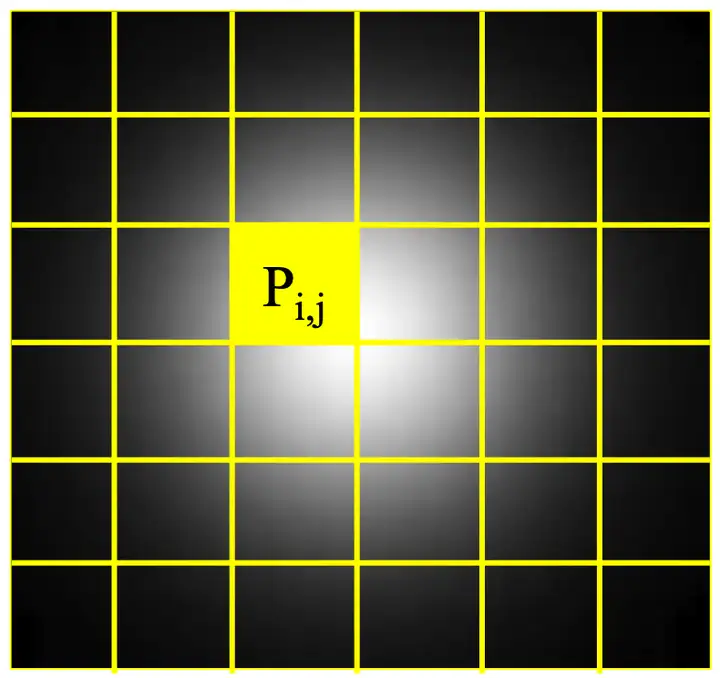
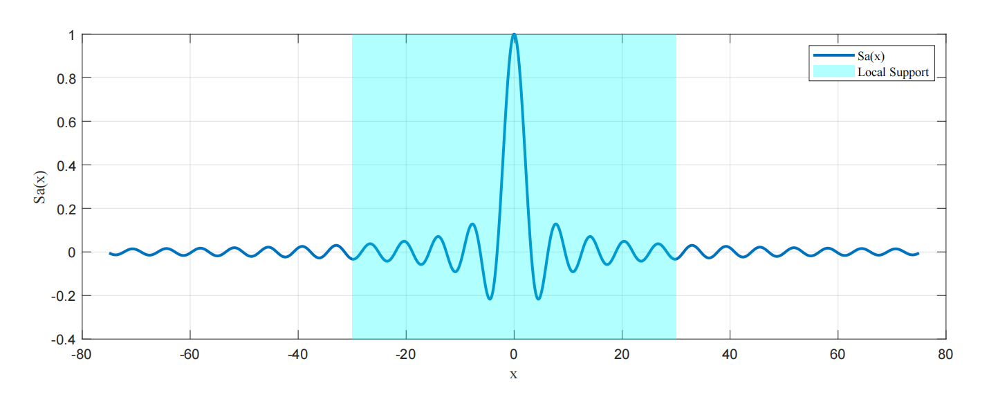
1. Local support: the regime of each 3D kernel is range-limited and not overlapped with other kernels on the ray.

   

   The attribute (e.g., color) in the local support region of a 3D kernel along a ray is assumed to be constant. Specifically, the $c(𝐱,ξ)$ over the line of sight (for all ξ) is constant, while other rays (i.e., 𝐱) passing through the kernel can have different colors. Hence, c(𝐱,ξ) can be put outside of the ray integral.

   $$g_c(𝐱) = ∑_{k∈IN} wₖ cₖ(𝐱) \left( ∫_{ξ=0}^L rₖ’(𝐱,ξ) ⋅ ∏_{j∈IN} e^{- wⱼ⋅∫_{μ=0}^ξ rⱼ’(𝐱,μ) dμ} ⋅dξ \right)$$

2. Assume the attenuation factor of voxels in a kernel along a ray is constant, i.e., the transmittance isn’t dependent on previous voxels passed through by the ray, but equals the accumulation of all voxels. Thus, the upper bound of the integral becomes L:

   $$\rm exp(-∫_{μ=0}^{ξ} f_c’(𝐱, μ) dμ) → exp(-∫_{μ=0}^{L} f_c’(𝐱, μ) dμ)$$

   In this way, the transmittance isn’t restricted by ξ of the outer rendering integral and can be pulled outside.

   $$g_c(𝐱) = ∑_{k∈IN} wₖ cₖ(𝐱) ( ∫_{ξ=0}^L rₖ’(𝐱,ξ)dξ ) ⋅ ∏_{j∈IN} e^{- wⱼ⋅∫_{μ=0}^L rⱼ’(𝐱,μ) dμ} $$

   The integral of opacities of all voxels rₖ’(𝐱,ξ) on the line of sight L belonging to a kernel is denoted as:

   $$ qₖ(𝐱) = ∫_{x₂=0}^L rₖ’(𝐱,x₂) dx₂ $$

   • qₖ(𝐱) is the footprint function for a 3D kernel $rₖ’(𝐱,x₂)$ in the ray space.

   • qₖ(𝐱) is a 2D function that specifies the contribution (total opacity) of a 3D kernel to a screen location.

     The 3rd dimension (x₂) of a kernel has been integrated out. Thus, inputting a 2D coordinates, it returns an attribute’s weight resulting from the corresponding kernel.

     (2023-12-31) The objects to be blended differ between EWA and NeRF.

     • (2024-01-04) In NeRF, points on a ray are composited, whereas EWA blends “line segments”. (refer to 八氨)

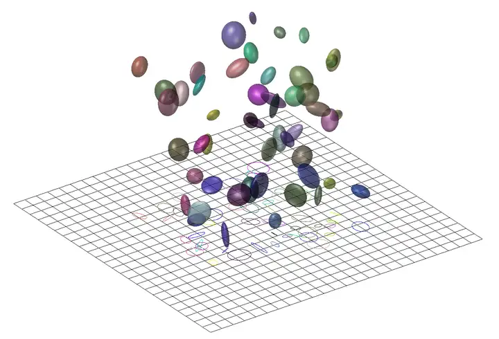
     • In EWA, scene voxels are grouped into different ellipsoids, and then rendering for ellipsoids, instead of volume-wise compositing. The scene element is a line integral of an ellipsoid, analogous to a particle in the volume rendering, thereby boosting efficiency.

     • In this ellipsoidal scenario, the alpha of each ellipsoid is the footprint function (opacity integral over the line of sight).

   • And 3D kernels in the dataset can be preintegrated before rendering.

     With the opacity precomputed, the alpha compositing is a 2D convolution over the line of sight L for splatting, whereas ray-casting needs 3D convolutions. Thus, splatting is more efficient.

   With this approximation, volume rendering equation becomes:

   $$g_c(𝐱) = ∑_{k∈IN} wₖ ⋅cₖ(𝐱)⋅ qₖ(𝐱) ⋅ ∏_{j∈IN} e^{- wⱼ⋅qⱼ(𝐱)} $$

3. Assume all kernels are ordered back to front (statements inconsistent in the paper), so that when computing the transmittance, only the opacities of kernels prior to the current kernel need to be accumulated.

   $$g_c(𝐱) = ∑_{k∈IN} wₖ ⋅cₖ(𝐱)⋅ qₖ(𝐱) ⋅ ∏_{j=0}^{k-1} e^{- wⱼ⋅qⱼ(𝐱)} $$

4. The exponential term is approximated by its 1st-order Taylor expansion based on $e^{-x} = 1-x$ evaluated at x=0:

   $$ e^{- wⱼ⋅qⱼ(𝐱)} \approx 1-wⱼ qⱼ(𝐱) \\ g_c(𝐱) = ∑_{k∈IN} wₖ ⋅cₖ(𝐱)⋅ qₖ(𝐱) ⋅ ∏_{j=0}^{k-1} (1-wⱼ qⱼ(𝐱)) $$

   $g_c(𝐱)$ is the splatting equation representing the continuous screen.

Consequently, with the above 4 assumptions, the point-based splatting becomes the same form as the NeRF-style volumetric rendering, because they’re both based on alpha compositing (image formation model). (Refer to 3DGS)

Combine Filter

Screen is a continuous 2D representation of the scene. A discrete image grid can be obtained by sampling it with an impulse train. To avoid aliasing when sampling the screen function, each projected 2D splat needs to be filtered to the Nyquist frequency of the output image by passing a proper loss-pass filter $h(𝐱)$.

$$ \begin{aligned} &\^g_c(𝐱) = g_c(𝐱) ⊗ h(𝐱) \\ &= ∫_{η=-∞}^{∞} ∑_{k∈IN} wₖ ⋅ cₖ(\bm η) ⋅ qₖ(\bm η) ⋅ ∏_{j=0}^{k-1} (1-wⱼ qⱼ(\bm η)) ⋅ h(𝐱-\bm η) d\bm η \\ &= ∑_{k∈IN} wₖ ⋅ ∫_{η=-∞}^{∞} cₖ(\bm η) ⋅ qₖ(\bm η) ⋅ ∏_{j=0}^{k-1} (1-wⱼ qⱼ(\bm η)) ⋅ h(𝐱-\bm η) d\bm η \\ \end{aligned} $$

• cₖ(𝛈) is the color (emission coefficient) of the ray point (𝛈,ξ) calculated relative to the kernel rₖ. It’s a function of rays 𝛈.

• qₖ(𝛈) is the contribution (total opacity) of the kernel rₖ to the screen point 𝛈.

• The cumulative product term is the transmittance (attenuation) of each voxel (𝛈,ξ) in the kerenel rₖ.

Because the color cₖ(𝛈) and the transmittance of a voxel (𝛈,ξ) in a kernel have no explicit formula to be integrated, two approximations are introduced to reach an analytical expression to compute.

1. Color of any voxel on any ray 𝛈 in the support region of a 3D kernel rₖ is a constant cₖ:

   $$cₖ(\bm η) = cₖ$$

2. Transmittance of each voxel in the kernel rₖ is a constant.

   $$∏_{j=0}^{k-1} (1-wⱼ qⱼ(\bm η)) \approx oₖ $$

   • The transmittance variation inside a 3D kernel is omitted, so the sole splatting equation can’t avoid edge aliasing, which needs to be solved by other techniques.

Therefore after filtering, the footprint function becomes band-limited in frequency domain:

$$∫_{η=-∞}^{∞} qₖ(\bm η) h(𝐱-\bm η)d\bm η$$

And the antialiased splatting equation (screen function):

$$ \begin{aligned} \^g_c(𝐱) &= g_c(𝐱) ⊗ h(𝐱) \\ &≈ ∑_{k∈IN} wₖ⋅cₖ⋅oₖ⋅∫_{η=-∞}^{∞} qₖ(\bm η) ⋅ h(𝐱-\bm η) d\bm η \\ &= ∑_{k∈IN} wₖ⋅cₖ⋅oₖ⋅ (qₖ ⊗ h)(𝐱) \end{aligned} $$

The formula can be interpreted as a weighted sum (combination, expectation) of footprint function in the 2D screen space. Thus, the primitives are the projected, prefiltered reconstruction kernels, so called ideal volume resampling filter:

$$ρₖ(𝐱) = cₖ⋅oₖ⋅(qₖ ⊗ h)(𝐱)$$

Instead of band limiting the output function $g_c(𝐱)$ directly, we band limit each footprint function qₖ separately.

(2023-11-26)

EWA Splats

The ideal volume resampling filter (splat primitive) is obtained after 3 steps: projection (viewing + projective transformation), footprint function, and convolving with a Gaussian loss-pass filter.

Gaussian will yields a Gaussian after affine transformations, convolving with another Gaussian, and integrating along one of its dimensions.

Therefore, 3D Gaussian is used as 3D reconstruction kernels (in object space) to produce an analytical expression of the 2D Gaussian resampling filter $ρₖ(𝐱)$ in screen space. So that splatting equation is an elliptical weighted average (EWA).

A reconstruction kernel centered at datapoint 𝐮ₖ in the object space is defined as the 3D Gaussian distribution with a mean vector 𝐮ₖ and a covariance matrix 𝐕ₖ:

$$rₖ(𝐮) = \frac{1}{(2π)^{3/2} det(𝐕ₖ)^{1/2}} e^{-½(𝐮-𝐮ₖ)^T 𝐕ₖ^{-1} (𝐮-𝐮ₖ)}$$

(2023-11-28)

Project Kernels

Project a 3D Gaussian distribution from object space to ray space through a viewing transformation and a projective transformation.

Viewing transformation φ

Transform a Gaussian distribution from source (object) space to camera space through an affine mapping: $𝐭=𝐖 𝐮+𝐝$. If 𝐖 is invertible, there is $𝐮 = 𝐖⁻¹(𝐭-𝐝)$.

Given a probability density function $f_𝐮$ of the variable 𝐮, and a linear mapping 𝐭=𝐖 𝐮+𝐝, by substituting the 𝐮 of $f_𝐮(𝐮)$ with 𝐖⁻¹(𝐭-𝐝), the result expression is a new distribution $f_𝐭$ represented in 𝐭’s space:

$$f_𝐭(𝐭) = \frac{1}{(2π)^{3/2} det(𝐕ₖ)^{1/2}} e^{-½(𝐖⁻¹(𝐭-𝐝)-𝐮ₖ)^T 𝐕ₖ^{-1} (𝐖⁻¹(𝐭-𝐝)-𝐮ₖ)}$$

• Clarify: Subscripts indicate which variable’s distribution the function is depicting. The argument in parentheses is the variable building the function (in the associate space).

On the other hand, to represent the PDF $f_𝐮$ in another space with a new variable, e.g., 𝐭 associating with $f_𝐮(𝐭)$, rather than the generic $f_𝐮(𝐮)$. After substituting variable, the result representation in 𝐭’s space is $f_𝐭(𝐭)$ as stated above.

But the scale is mismatched. According to the Change of Variables theorem, the “absolute value of the determinant of the Jacobian matrix” must be multiplied as a scaling factor to align different units between 𝐭 and 𝐮.:

$$f_𝐮(𝐭) = f_𝐭(𝐭) ⋅|det(\frac{∂𝐮}{∂𝐭})| = f_𝐭(𝐭)⋅ |det(𝐖⁻¹)|$$

And the new variable 𝐭’s PDF can be written as: $$f_𝐭(𝐭) = \frac{1}{|det(𝐖⁻¹)|} f_𝐮(𝐭)$$

, corresponding to the equation (21) in the paper: $G_𝐕^n (ϕ⁻¹(𝐮) - 𝐩) = \frac{1}{|𝐌⁻¹|} G_{𝐌 𝐕 𝐌ᵀ}^n(𝐮-ϕ(𝐩))$

• (2023-11-28) doubt: I’m confused in eq. (21), is the LHS the $f_𝐭(𝐭)$? Why do they care the unscaled distribution?

• (2023-12-02) If the |det(J)| is missing and just substituting variable, the new distribution $f_𝐭(𝐭)$ can’t be written as a Gaussian (?). So, the author used the transformed “non-“Gaussian divided by the factor, such that the new distribution is a Gaussian as well.

• (2023-12-31) I forgot the meaning of the above comment on 2023-12-02. The eq. (21) can be understood as:

  1. Given an affine mapping: 𝐮 = 𝐌 𝐱+c = ϕ(𝐱), and define its inverse as: 𝐱 = 𝐌⁻¹(𝐮-c) = ϕ⁻¹(𝐮)

  2. Given the distribution of 𝐱 is $G_𝐕^n (𝐱 - 𝐩)$, after applying the affine mapping 𝐌 𝐱+c, the mean and variance will become: ϕ(𝐩) and 𝐌 𝐕 𝐌ᵀ. So the new distribution is represented as $G_{𝐌 𝐕 𝐌ᵀ}^n (𝐮 - ϕ(𝐩))$.

  3. According to Change of Variables, the relations are:

     $$ Gⁿ_𝐕(𝐱-𝐩) \overset{substitute}{→} Gⁿ_𝐕(ϕ⁻¹(𝐮) - 𝐩) \overset{times |det(J)|}{→} G_𝐕^n(ϕ⁻¹(𝐮) - 𝐩) |𝐌⁻¹| = G_{𝐌 𝐕 𝐌ᵀ}^n (𝐮 - ϕ(𝐩)) $$

     So the eq.(21) is indeed the unscaled transformed Gaussian in another space.

     doubt: The unscaled, merely variable-changed distribution $Gⁿ_𝐕(ϕ⁻¹(𝐮) - 𝐩)$ is also a Guassian (?), as the 3 axes are stretched by the affine mapping linearly and separately, so the overall shape of Gaussian will be kept. And the |det(J)| is just a scalar coefficient ensuring consistent area quantity.

Similarly, the case of projecting a kernel from source space into camera space ($𝐭=𝐖 𝐮+𝐝$) is changing mean vector and covariance matrix:

$rₖ(𝐭)$ is the transformed representation of the kernel $k$ in the camera space, matching the above $f_𝐮(𝐭)$, so it equals the variable-changed $rₖ(𝐮)$ multiplied with $|det(∂𝐮/∂𝐭)|$:

$$ \begin{aligned} &rₖ(𝐭) = rₖ(𝐖⁻¹(𝐭-𝐝)) ⋅ |det(𝐖⁻¹)| \\ &= \frac{1}{(2π)^{3/2} \sqrt{det(𝐕ₖ)} |det(𝐖)|} e^{-½(𝐖⁻¹(𝐭-𝐝)-𝐮ₖ)ᵀ𝐕ₖ⁻¹(𝐖⁻¹(𝐭-𝐝)-𝐮ₖ )} \\ &= \frac{1}{(2π)^{3/2} \sqrt{det(𝐕ₖ)} |det(𝐖)|} e^{-½(𝐖⁻¹(𝐭-𝐝-𝐖𝐮ₖ))ᵀ𝐕ₖ⁻¹(𝐖⁻¹(𝐭-𝐝-𝐖𝐮ₖ) )} \\ &= \frac{1}{(2π)^{3/2} \sqrt{det(𝐕ₖ)} |det(𝐖)|} e^{-½(𝐖⁻¹(𝐭-(𝐖𝐮ₖ+𝐝)))ᵀ𝐕ₖ⁻¹(𝐖⁻¹(𝐭-(𝐖𝐮ₖ+𝐝)) )} \\ &= \frac{1}{(2π)^{3/2} ⋅ \sqrt{det(𝐕ₖ)} ⋅ |det(𝐖ᵀ)|^½ ⋅ |det(𝐖)|^½} \\ &\quad ⋅ e^{-½(𝐭-(𝐖𝐮ₖ+𝐝))ᵀ(𝐖⁻¹)ᵀ𝐕ₖ⁻¹𝐖⁻¹(𝐭-(𝐖𝐮ₖ+𝐝)) } \\ &= \frac{1}{(2π)^{3/2} \sqrt{|det(𝐖 𝐕ₖ 𝐖ᵀ)}|} e^{-½(𝐭-(𝐖𝐮ₖ+𝐝))ᵀ(𝐖ᵀ)⁻¹𝐕ₖ⁻¹𝐖⁻¹(𝐭-(𝐖𝐮ₖ+𝐝)) } \\ &= N(𝐖𝐮ₖ+𝐝, 𝐖 𝐕ₖ 𝐖ᵀ) \end{aligned} $$

Hence, after performing an affine transformation, the distribution in the new space has a new mean vector 𝐖𝐮ₖ+𝐝, i.e., the original mean 𝐮ₖ is shifted by the affine mapping, and the variance matrix becomes 𝐖 𝐕ₖ 𝐖ᵀ.

• Derivation refers to: Linear Transformation of Gaussian Random Variable (Found by DDG with keywords: “affine transform for Gaussian distribution”)

• Fact: $(Wᵀ)⁻¹ = (W⁻¹)ᵀ$

• Affine property for x~N(0,1): STAT 830 The Multivariate Normal Distribution - SFU

• The Multivariate Gaussian Distribution - Stanford

Projective transformation ϕ

• (2024-01-04) Summary: The non-linear projective transformation is approximated via Taylor expansion.

In this paper, a 3D point (x,y,z) is projected onto a plane perspectively as follows: the x, y coordinates are divided by z, and the z value is then reset to the Euclidean norm $‖𝐭‖$ for object culling.

In this way, points in the camera space are transformed into the 3D ray space.

$$ \begin{bmatrix}x₀ \\ x₁ \\ x₂ \end{bmatrix} = ϕ(\begin{bmatrix}t₀ \\ t₁ \\ t₂ \end{bmatrix}) = \begin{bmatrix}t₀/t₂ \\ t₁/t₂ \\ \|(t₀,t₁,t₂)ᵀ\| \end{bmatrix} $$

• After perspective division with pixel coords obtained, x₂ is supposed to be 1, but it’s assigned with ‖𝐭‖₂.

• Denote the L2 norm of 𝐭 as l: $‖(t₀,t₁,t₂)ᵀ‖ = l = \sqrt{t₀²+t₁²+t₂²}$, i.e., the magnitude of the line connecting a point 𝐭 to the projection center on the screen.

• The dpeth is not confined to [-1,1] like NDC. The points on a single ray all have the same (t₀,t₁)ᵀ, thus, the depth $x₂=\sqrt{t₀²+t₁²+t₂²}$ only depends on t₂.

• Although $y=\sqrt{1+x²}$ is not linear, it’s approaching linear: $y=x$ as x grows.

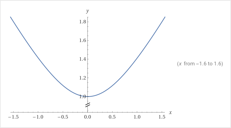  (plot by Perplexity-Wolfram)

• By using the L2 norm of the camera-space coordinates 𝐭 as the depth, the evenly sampled points on the line of sight in the ray space will almost remain evenly spaced after this non-linear projection (due to perspective division) from 𝐭 to 𝐱, close to directly using the t₂ of camera space as the depth:

  • (2024-01-01) Unlike directly using t₂ as the depth in the ray space, with which the uniform intervals can be exactly kept (as perspective projection with homogeneous coords is linear), this approach considers both t₀ and t₁.

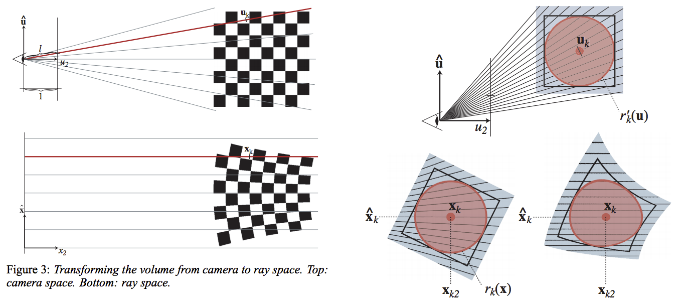
• After viewing transformation, it is the kernels that are viewing the screen. Thus, the screen seen by a kernel is perspective (i.e., near large, far small, as shown below Fig.3 bottom) after projective transformation. Each ray emitted from the kernel is parallel to each other in the ray space.

  

  (2024-01-06)

  • The transformation ϕ from camera space to ray space should be understood as the datapoints are projected into the ray space (or the screen by disregarding the x₂) perspectively, because we want to display 3D world in a 2D plane. (Note: x₂ is independtly assigned beside the screen coordinates x0,x1, so ray space = screen + x₂.)

    Shortly, the near-large-far-small effect is desired. But it’s a nonlinear function, so its linear approximation is applied to simulate those “curves”. As shown in Fig. 9, the correct perspective curving effects (bottom-right) aren’t accurately represented by an linear projection (bottom-left). Intuitively, one might think that all points are using a common depth value, but for the exact perspective projection, each point should use its individual depth.

  • In addition, the x₂ (‖𝐭‖₂, depth in the ray space) can be disregarded, because the datapoints have already been projected onto the screen, i.e., (x₀,x₁). The existence of ray space may just for introducing the footprint function (ray integral). The “projective transformation ϕ” is solely assigning x₂ based on the perspective projection.

    The statement that “rays are parallel” may be misleading, as the perspective projection (x,y divided by z) has been performed, and one can focus on the screen directly. “Parallel” doesn’t mean that the kernel is projected onto the screen orthogonally, because they already are on the screen. The ray space is set for defining the footprint function of each kernel as an integral along a certain viewing ray, which remains a straight line in the 3D ray space after perspective projection due to the linear approximation.

    And it is the viewing ray that will be orthogonally projected onto the screen. Thereby, the ray integral in the 3D ray space becomes a line integral on the 2D screen plane, i.e., an integral for a 2D Gaussian.

    • (2024-01-07) The 3D Gaussian integral in the ray space equals the 2D Gaussian integral in the screen space (?), because I think that the “voxels” perpendicular to a pixel at different depths are replicas of that pixel, which is projected by a certain kernel.
    • The depth dimension x₂ is ‖𝐭‖₂, which is independent to x0, x1. So ray space is “orthogonal” to the screen.
    • In other words, a screen pixel is a summation of only kernels that overlaps with it, because object-space 3D Gaussian have already been projected perspectively onto the screen (corresponding to 2D center and covariance matrix), and the ray space is constructed after that projection as “rays space = screen + x₂”.

    In short, ray space is for viewing rays, not for datapoints.

    (2024-01-07)

    • The viewing ray is only used to compute each kernel’s opacity, which is the contribution coefficient to the target pixel’s color.

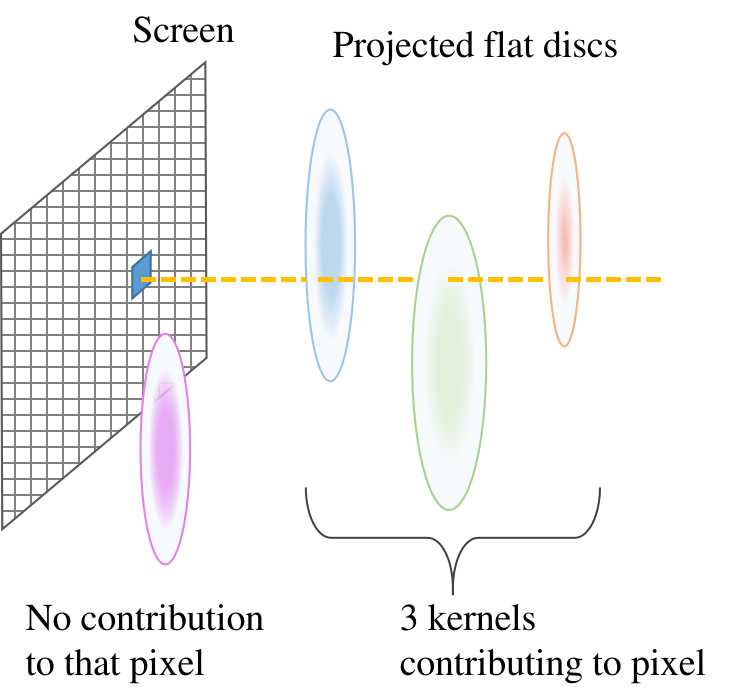
    • Kernels contributing to the target pixel are determined by whether a kernel overlaps with the pixel after being thrown onto the screen. In essence, the contributing kernel in the ray space is located on the perpendicular line to the target pixel, and its squashed flat disc covers the target pixel.

      

    • The role of viewing rays in splatting differs from volume rendering, where a viewing ray yields a pixel color, but in splatting, color is generated from kernels and a viewing ray determines the weights of kernels.

    (2024-01-22)

    • The 2D location (x₀,x₁) of a Gaussian center on the screen and the 2D covariance matrix are determined by perspective projection, while the opacity of a Gaussian is determined by computing the integral over x₂ along the viewing ray in the 3D ray space.

However, this perspective projection is not affine (linear) because the depth t₂ is divided and x₂ is reassigned. Therefore, the first-order Taylor expansion of this transformation matrix is used as its linear approximation.

• (2024-01-05) The reassignment of x₂ is not the reason for the approximation. x₂ is just used for integration along the viewing ray. And after approximation, the shape of the 2D Gaussian doesn’t depend on depth, which (the 3rd row, col) will be omitted to obtain the 2D covariance matrix of the projected 2D ellipse.

The Jacobian matrix of ϕ(𝐭) is:

$$ (\begin{bmatrix}t₀/t₂ \\ t₁/t₂ \\ ‖(t₀,t₁,t₂)ᵀ‖ \end{bmatrix})’= 𝐉 = \begin{pmatrix} 1/t₂ & 0 & -t₀/t₂² \\ 0 & 1/t₂ & -t₁/t₂² \\ t₀/l & t₁/l & t₂/l \end{pmatrix} $$

The first-order Taylor expansion evaluated at the kernel center point 𝐭ₖ is called the local affine approximation:

$$ \begin{aligned} & ϕₖ(𝐭) = ϕ(𝐭ₖ) + 𝐉ₖ ⋅ (𝐭-𝐭ₖ) \\ \\ & 𝐉ₖ = \frac{∂ϕ}{∂𝐭}(𝐭ₖ) = \begin{pmatrix} 1/tₖ,₂ & 0 & -tₖ,₀/tₖ,₂² \\ 0 & 1/tₖ,₂ & -tₖ,₁/tₖ,₂² \\ tₖ,₀/‖𝐭ₖ‖ & tₖ,₁/‖𝐭ₖ‖ & tₖ,₂/‖𝐭ₖ‖ \end{pmatrix} \end{aligned} $$

• (2024-01-10) If the 𝐭 is 𝐭ₖ, (𝐭-𝐭ₖ). So, there is no approximation, the projection of 𝐭ₖ is exact ϕ(𝐭ₖ). This is what the following sentence in the paper means.

  “As illustrated in Fig. 9, the local affine mapping is exact only for the ray passing through tk or xk, respectively.”

  And for the point far away from the Guassian center, the approximation result has a noticeble deviation from the actual case, as (𝐭-𝐭ₖ) is large.

By concatenating the viewing transform φ(𝐱) and projective transform ϕ(𝐭), the conversion for a point 𝐮 in source space to 𝐱 in ray space is an affine mapping 𝐦(𝐮):

$$𝐭 = φ(𝐮) = 𝐖 𝐮+𝐝 \\ 𝐱 = 𝐦ₖ(𝐮) = ϕₖ(𝐭) = ϕ(𝐭ₖ) + 𝐉ₖ ⋅ (𝐭-𝐭ₖ) \\ = 𝐱ₖ + 𝐉ₖ ⋅ (𝐖 𝐮+𝐝 -𝐭ₖ) = 𝐉ₖ⋅𝐖 𝐮 + 𝐱ₖ + 𝐉ₖ⋅(𝐝-𝐭ₖ)$$

Therefore, for this compound affine mapping, the multiplier is $𝐉ₖ⋅𝐖 $, and the bias is $𝐱ₖ + 𝐉ₖ⋅(𝐝-𝐭ₖ)$.

According to the aforementioned viewing transformation derivation, the kernel in the 3D ray sapce rₖ’(𝐱) has a shifted mean 𝐮ₖ and a scaled variance 𝐕ₖ:

$$ rₖ’(𝐱) ∼ N(𝐦(𝐮ₖ), 𝐉ₖ𝐖 𝐕ₖ 𝐖 ᵀ𝐉ₖᵀ) $$

• (2023-12-02) doubt: Does the eq. (30) mean that the unscaled representation in ray space is the desired projected kernel?

  The normalization factor of the transformed Gaussian is canceled, so that its integral isn’t a unit. Is that they want?

Integrate Kernels

The footprint function is an integral over the voxels in a 3D kernel along the ray.

Given a 3D kernel in the ray space rₖ’(𝐱) as above, the footprint function is the integral over depth:

Convolve with Filter

The anti-aliased splatting equation is achieved by using the band-limited footprint function under 2 assumptions described above.

Convolving the footprint function with a Gaussian low-pass filter: