下一代国际华人青年学子面对面 第6期 2022年10月20日 周四
Overview
- Research work
- Suggestions for graduate student (1st year)
Research Contribution:
-
Non-iterative learning strategy for training neural networks including single-layer networks, multi-layer networks, autoencoders, hierarchical networks, and deep networks. All the related publications in this category are my first-author papers
-
The proposed methods for pattern recognition related applications: Image Recognition, Video Recognition, Hybrid System Approximation, Robotics System Identification, EEG-brain Signal Processing. Most the related publications in this category are co-author papers with my HQPs.
My research works
In the past 10 years, the works about Artificial neural networks:
| Theoretical Contributions to ANN | Machine Learning based Applications |
|---|---|
| Single-layer network with non-iterative learning | Data Analysis and Robotics System Identification (Ph.D.) |
| Hierarchical NN with Subnetwork Neurons | Image Recognitions (Post Doctoral Fellow) |
| Deep Networks without iterative learning | Pattern Recognition (since 2018) |
Ⅰ. Single-layer network with non-iterative learning
Starting with a small idea
The labtorary mainly studies robots, control, mechanics. After 2008 Chinese Winter Storms, they got funding for creating Powerline De-icing robots.
The supervisor (Yaonan Wang): “Can you find a Neural Network for Identifying Robotics Dynamic Systems?” (in 2009 winter)
Later, I found the following paper: “Universal approximation using incremental constructive feedforward networks with random hidden nodes”, By Huang, Guang-Bin et.al (Cannot be found on IEEE) version on elm portal
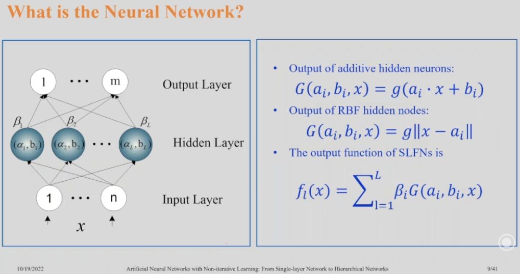
What is the Neural Network?
Single hidden layer feedforward NN:
- Output of additive hidden neurons: G(𝐚ᵢ, bᵢ, 𝐱) = g(𝐚ᵢ⋅𝐱+bᵢ)
- Output of RBF hidden nodes: G(𝐚ᵢ, bᵢ, 𝐱) = g‖𝐱-𝐚ᵢ‖
- The output function of SLFNs is: fₗ(𝐱) = ∑ₗ₌₁ᴸ 𝛃ᵢ⋅G(𝐚ᵢ, bᵢ, 𝐱)
Network training
Advantage: Approximate unknown system through learnable parameters.
Mathematical Model:
-
Approximation capability: Any continuous target function f(x) can be approximated by Single-layer feedforward network with appropriate parameters (𝛂,♭,𝛃). In other words, given any small positive value e, for SLFN with enough number of hidden nodes, we have:
‖f(𝐱)-fₗ(𝐱)‖ < e -
In real applications, target function f(𝐱) is usually unknown. One wishes that unknown f could be approximated by the trained network fₗ(𝐱).
What is Extreme Learning Machine?
Feed forward random network without using BP to train, such that it has a good real-time performance. And it fits the real-time robot task exactly.
B-ELM
(2011) “Bidirectional ELM for regression problem and its learning effectiveness”, IEEE Trans. NNLS., 2012 paper
(23-02-10) This the inception of his subnetwork series work, and I was supposed to read this brief firt. paperNote
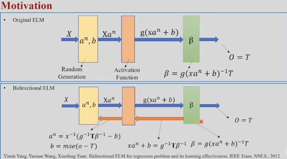
Motivation
-
Original ELM has 3 kinds of parameters: 𝐚 is called the “input weights”, b is the bias, 𝛃 is the “output weights”, which are consistent with earlier feedfoward network, though current single-layer feedfoward network has removed the 𝛃.
The 1st layer in ELM is generated randomly and the 2nd layer is constructed based on Moore-Penrose inverse without iteration.
flowchart LR in((X)) --> lyr1["Layer1:\n 𝐚ⁿ, b\n Random\n Generated"] --> weightSum1(("X⋅𝐚ⁿ + b")) --> act[Activation\n Function\n g] --> z(("g(X⋅𝐚ⁿ+b)")) --> lyr2["Layer2:\n 𝛃"] --> weightSum2(("O =\n 𝛃⋅g(X⋅𝐚ⁿ+b)\n =T")) -.->|"𝛃 =\n g(X⋅𝐚ⁿ+b)⁻¹T"| lyr2 classDef lyrs fill:#ff9 class lyr1,act,lyr2 lyrs; -
Bidirectional ELM
In original ELM, the 𝐚ⁿ,b are random numbers, but they can be yield if pulling the error back further, that is doing twice more inverse computation. Therefore, in order to calculate the 𝐚ⁿ,b, there are 3 times inverse computation: for output weights 𝛃, activation function g(⋅) and activation z (X⋅𝐚ⁿ+b) respectively.
%%{ init: { 'flowchart': { 'curve': 'bump' } } }%% flowchart LR in((X)) --> lyr1["Layer1:\n 𝐚ⁿ, b\n Random\n Generated"] --> weightSum1(("X⋅𝐚ⁿ + b")) --> act[Activation\n Function\n g] --> z(("g(X⋅𝐚ⁿ+b)")) --> lyr2["Layer2:\n 𝛃"] --> out(("O =\n 𝛃⋅g(X⋅𝐚ⁿ+b)\n =T")) -.->|"𝛃 =\n g(X⋅𝐚ⁿ+b)⁻¹T"| lyr2 classDef lyrs fill:#ff9 class lyr1,act,lyr2 lyrs; out -.-> |"X⋅𝐚ⁿ+b =\n g⁻¹ T 𝛃⁻¹"|weightSum1 out -.-> |"𝐚ⁿ =\n X⁻¹ (g⁻¹ T 𝛃⁻¹ -b ),\n b = mse(O-T)"|lyr1- 𝛃 = [g(X⋅𝐚ⁿ+b)]⁻¹T
- X⋅𝐚ⁿ+b = g⁻¹ T 𝛃⁻¹
- 𝐚ⁿ = X⁻¹ (g⁻¹ T 𝛃⁻¹ -b ), and b = mse(O-T)
The error is surprisingly small even with few hidden nodes. Compared with the original ELM, the required neurons in this method are reduced by 100-400 times, and the testing error reduced 1%-3%, and also the training time reduced 26-250 times over 10 datasets.
Major differences
| Randomized Networks | Bidirectional ELM | |
|---|---|---|
| Classifier | ELM; Echo State Netowrk; Random Forest; Vector Functional-link Network |
Only works for regression task |
| Performance | Similar performance; Faster speed; Less required neurons |
|
| Learning strategy | (Semi-)Randomized input weights; Non-iterative training; Single-layer network |
Non-iterative training; Single-layer network; Calculated weights in a network |
Ⅱ. Hierarchical NN with Subnetwork Neurons
Single-Layer Network with Subnetwork Neurons
In 2014, deep learning is becoming popular. How to extend the B-ELM as a multi-layer network?
“Extreme Learning Machine With Subnetwork Hidden Nodes for Regression and Classification”.
paper; paperNote
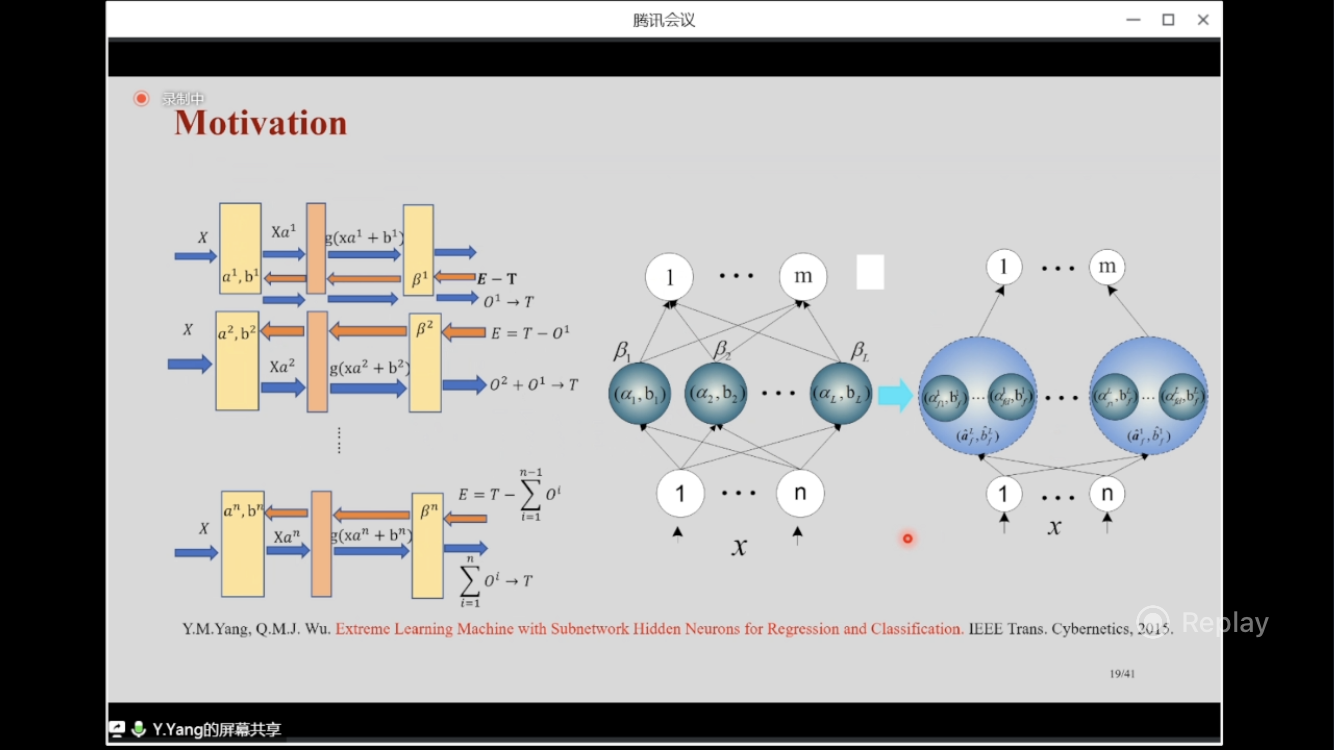
Motivation
Pull the residual error back to multiple B-ELMs sequentially:
Dotted links are computation with inverse. Cyan links is the second feedforward using the updated parameters to give a trustworthy result O¹. The objective is to approach the target T, so there is a residual error E=T-O¹. Then another B-ELM (with same structure) is used to reduce the error continuously. And this time, the prediction is O²+O¹, which is the approximation of T. Here, the residual error is E=T-(O²+O¹)
Repeatedly pulling the residual error to a new B-ELM N times is equivalent to N SLFNs. But B-ELM is fast without iteration and less computation with a few hidden nodes in each SLFN.
Based on original SLFN structure, each node contains a SLFN.
Two-Layer Network with Subnetwork Neurons
(2015) How to extend the Single-layer network with subnetwork nodes system to a two-layer network system?
A general two-layer system was built in paper: “Multilayer Extreme Learning Machine with Subnetwork Hidden Neurons for Representation Learning” paper; paperNote
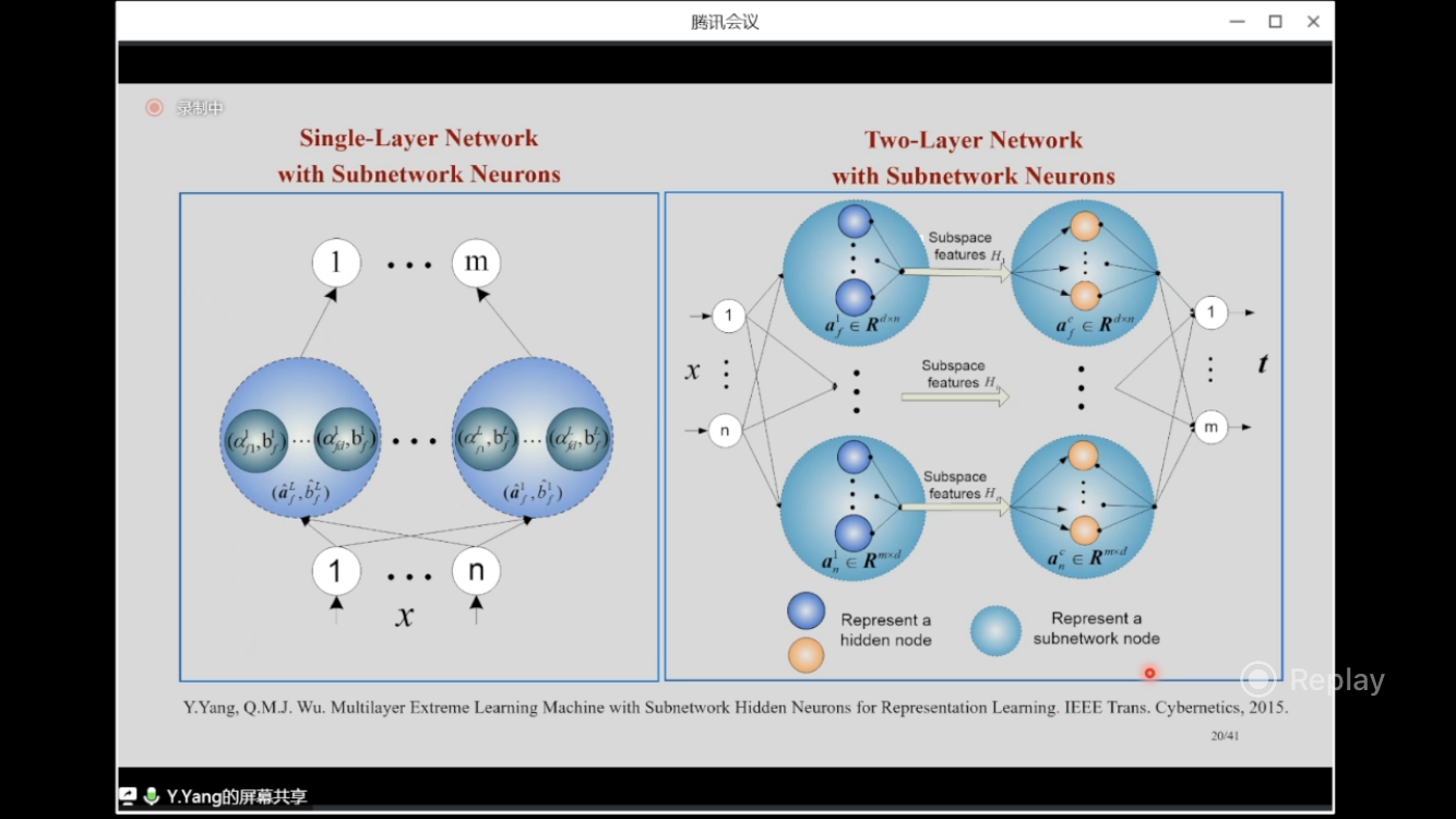
Though it only contains two “general” layers, this system includes hundreds of networks, and it’s fast due to the modest quantity and no iteration.
Compared with ELM and B-ELM, it got better performance over 35 datasets:
| Classification (vs ELM) | Regression (vs B-ELM) | |
|---|---|---|
| Required Neurons | Reduced 2-20 times | Reduced 13-20% |
| Metrics | Accuracy increase 1-17% | Testing error reduced 1-8% |
| Training Speed | faster 25-200times | faster 5-20% |
Two-layer network system can perform image compression or reconstruciton, etc. This method is better than Deep Belief Network on small datasets. But it’s inferior than deep learning with transfer learning technics on huge datasets.
Hierarchical Network with Subnetwork Neurons
“Features combined from hundreds of mid-layers: Hierarchical networks with subnetwork nodes” IEEE Trans. NNLS, 2019. paper
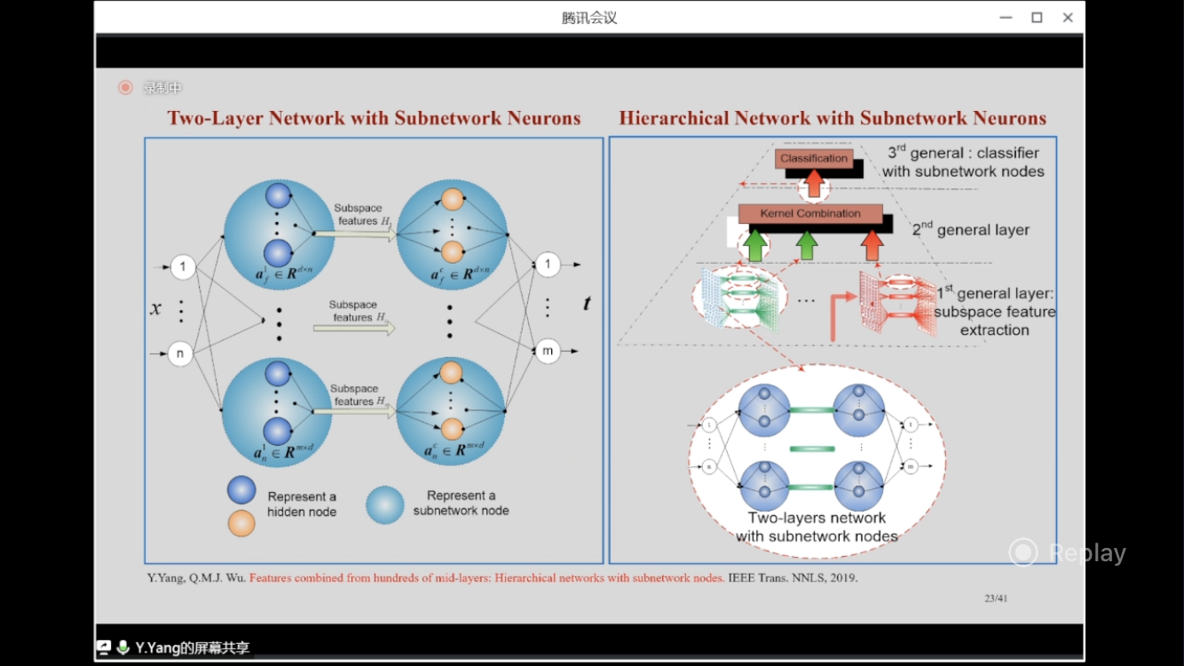
From a single-layer network with subnetwork neurons to the multi-layer network, and then to a neural network system, these 3 papers cost 5 years or so.
Compared with deep learning network, it’s extremely fast and performs well on small datasets, like Scene15, Caltech101, Caltech256. But for large datasets, deep learning is the winner.
“Somewhat regretfully, I turned to deep learning a bit late. But been hesitant to do research along this approach.”
Major differences between ours and Deep Networks
| SGD based methods in DCNN | Moore-Penrose inverse matrix based methods | |
|---|---|---|
| Hyper params | lr; momentum; bs; L2 regulariation; epochs | L2 regularization (non-sensitive) |
| Performance | higher performance in Computer Vision tasks (with huge datasets); GPU-based computation resource; More parameters; More required training time |
Faster learning speed/less tuning; Promising performance in Tabular Datasets; Less over-fitting problem. |
Ⅲ. Deep Networks without iterative learning
Since 2018: How to combine the non-iterative method (M-P inverse matrix) with deep convolutional network to gain advantages? This took 2-3 years.
This is the age of Deep Learning.
-
Interesting 20 years of cycles
- Rosenblatt’s Perceptron proposed in mid of 1950s, sent to “winter” in 1970s.
- Back-Propagation and Hopfield Network Proposed in 1970s, reaching research peak in mid of 1990s.
- Support vector machines proposed in 1995, reaching research peak early this century.
-
There are exceptional cases:
- Most basic deep learning algorithms proposed in 1960s-1980s, becoming popular only since 2012 (for example, LeNet proposed in 1989).
ImageNet pushed deep learning, because only when the huge network structure of deep learning meets the matched huge dataset, it can achive good performance.
The success of deep learning enlist three factors: 1. NN structure and algorithm; 2. Big data; 3. GPU availability.
Hundreds of layers result in tedious training time. “The study intensity is infinitely small and the study duration is infinitely large.”
“The improvement space of deep neural network is limited. So can we introduce non-iterative learning strategies for training deep networks”
Training speed is more important for scientific research than accuracy. And also it’s necessary to reduce the dependence on GPUs and the involvement of undeterministic hyper parameters (lr,bs,…)
Retraining DCNN with the non-iterative strategy
(2019): “Recomputation of the dense layers for the performance improvement of DCNN.” IEEE TPAMI, 2020. link
Motivation
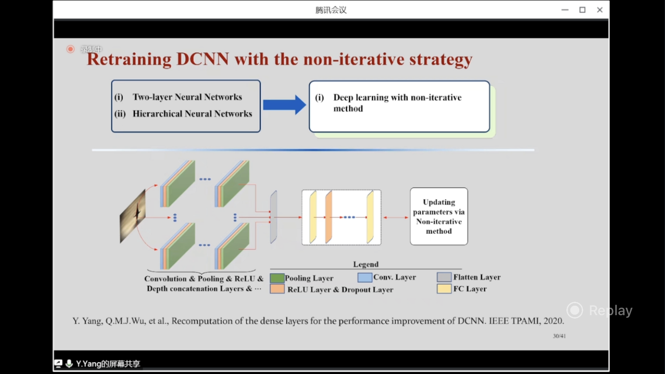
In a DCNN, the first few layers are convolutional layers, maxpooling, then there’re 3 or 1 dense layer.
If I cannot train all of the hundreds layers in my non-iterative method, can I train only certain layers that are easy trained with my method, rather the SGD?
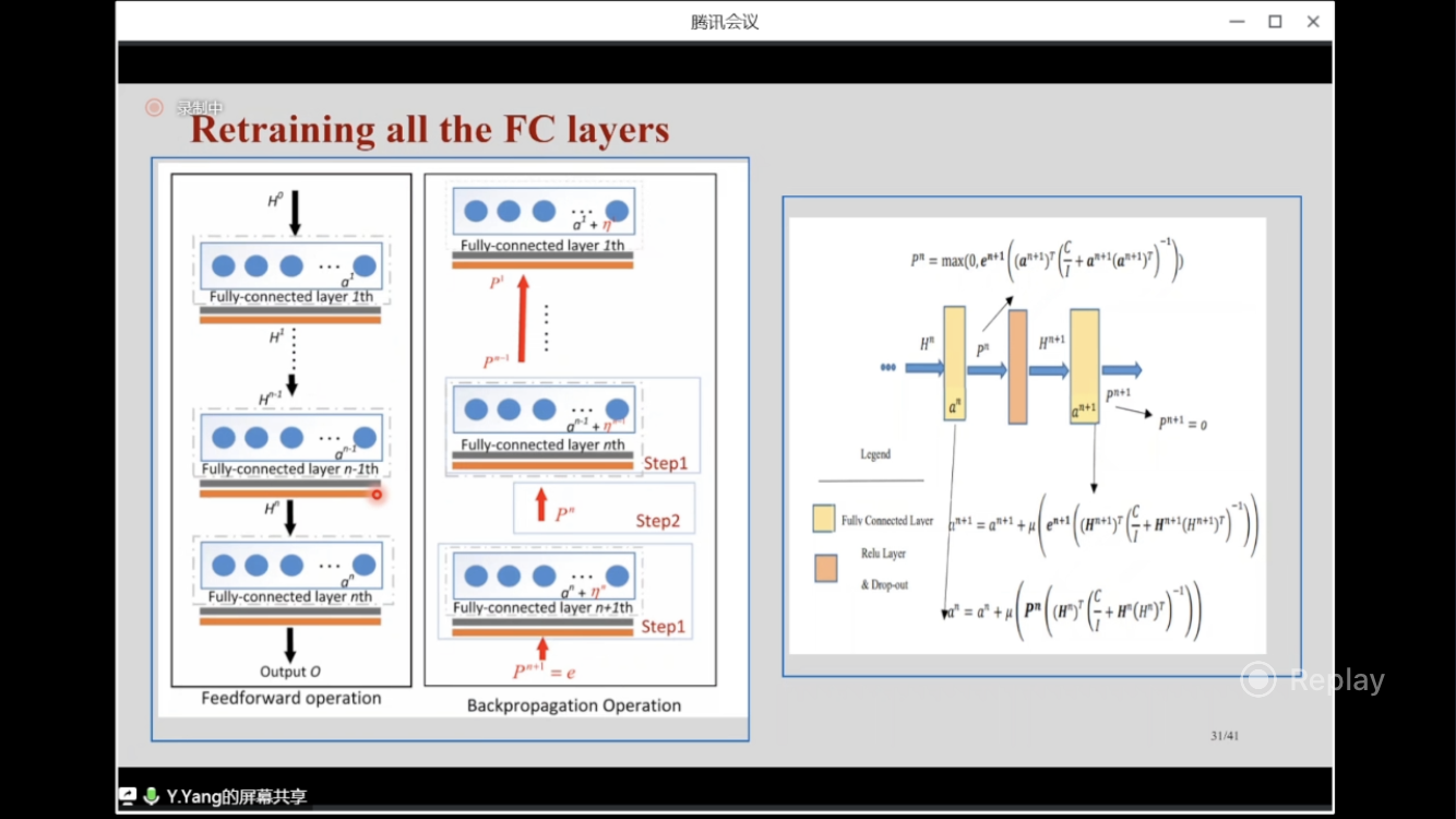
Only the fully-connected layers are trained by non-iterative method (inverse matrix), and the rest of layers are trained by gradient descent (SGD, SGDM, Adam).
On some medium-size datasets(CIFAR10, CIFAR100, SUN397), this approach brought a moderate improvement because there are only 3 dense layer out of a 50/100-layer network (most of layers are trained with SGD), but speeds up the training.
One layer can be trained within 1-2 seconds.