memo: Vis | Planar Homography

(2024-05-16)

Homography 是把一张照片变到另一个视角下

ex: 桌子上放着一张照片，从不同视角去看，除了正视，从其他视角看，看到照片里的内容就变形了。
- 注意：必须是照片，不要关注照片里的 3D 物体。 Homography 就是描述从不同角度看照片，看到的照片的样子。不论你从哪看，它就只是一个平面，所以斜着看照片，上面的内容就会拉伸收缩：比如上面的字放大缩小，一个正方形变成梯形。变换视角时，不会出现物体间的遮挡，因为只是在分析一个平面。

Homography warps two images to a common plane, or maps a pixel from a camera plane to another camera plane.

A pixel can be mapped to another camera because the 2 pixels are the projections of a common 3D point.
Homography warps the images captured from different angles, observing a common plane at a certain depth, to a unified viewpoint for stitching or other applications.
A homography corresponds to only one depth. If the image doesn’t only capture a plane at a certain depth, the part with a deviated depth will be distorted in the warped image. Thus, solving homographies requires specifying depth.
Homography relation is built based on the pose transformation between two cameras, and a depth embodied by a co-observed point or a co-observed plane. Or it can be sovled from 4 pairs of matched pixels.
Specifically, two cameras are connected via the 2 camera-space coordinates conversion for a depth-known co-observed 3D point.
1. The conversion can be represented by two camera’s poses in the world space, or the direct transformation from one camera to the other.
2. The depth of the co-observed 3D point can be given by specifying either the z-coordinate directly or a plane (𝐧,d) indirectly.
(2023-12-19) Two scenarios for homography: stitching images based on a co-observed plane, and transferring viewpoint for a plane surface. They both rely on the observed plane.

Two Cameras

The homography matrix is solved based on matching points in a pair of images.

$$ 𝐲₁ = 𝐏₁ ⋅ 𝐐 \\ 𝐲₂ = 𝐏₂ ⋅ 𝐐 \\ 𝐲₂ = 𝐏₂ ⋅ 𝐏₁⁻¹ * 𝐲₁ $$

𝐏 is the projecting operation that converts a world coordinates of a point 𝐱 to pixel coordinates 𝐲.

$𝐏 = 𝐊[𝐑|𝐭]$ and $𝐏⁻¹ = [𝐑|𝐭]⁻¹𝐊⁻¹$
𝐏₂ ⋅ 𝐏₁⁻¹ is the homography matrix.
Besides 𝐊[𝐑|𝐭], the z-coordinate of covisible point 𝐐 (or the “distance from camera center to plane” d) is necessary.

Since the inverse intrisics $𝐊⁻¹ ⋅(u,v,1)ᵀ$ solely can’t determine a unique 3D point as z has been canceled when $(u,v,1)ᵀ=\frac{1}{z}⋅𝐊⁻¹ ⋅ (x,y,z)ᵀ$, the z must be specified at first. 5

$$ (x,y,z)ᵀ = 𝐊⁻¹ ⋅z ⋅(u,v,1)ᵀ $$

If assuming camera’s z-axis is perpendicular to the observed plane, then z is indeed $d$. Thus, the z-retained coordinates of the pixel 𝐲₁ is (ud,vd,d), such that $𝐊⁻¹ ⋅d⋅(u,v,1)ᵀ$ is a unique 3D point in the camera space.
- Recall the NeRF’s sampling points (get_rays_np): meshgrid as pixel coordinates → divided by focal (with z=1) to be in camera space → @c2w to be in world space → z vals sampling
  
  Thus $𝐊⁻¹ ⋅(u,v,1)ᵀ$ only determines the viewdir, not a 3D point.
Then, roll back it to world space and project to the other camera to get the pixel 𝐲₂.

$$ 𝐲₂ = 𝐊₂[^{𝐑₂ \quad 𝐭₂}_{0 \quad 1}] [^{𝐑₁ \quad 𝐭₁}_{0 \quad 1}]⁻¹𝐊₁⁻¹ ⋅d⋅𝐲₁ $$

Overview: Plane1 → camera1 → world space → camera 2 → plane 2
However, if either 𝐐’s $z$ (or the distance $d$), or poses of two cameras is unknown, the 3x3 homography matrix can be solved from 4 pairs of matching pixels.

(2023-12-04)

Basis Changes

Refer to Planar homographies - Department of Computer Science, University of Toronto

In a “meta space” holding two cameras, for example the world space, a ray emitted from the world origin passed through 2 world points 𝐦, 𝐧 locating on 2 planes separately.

$\vec{a₀}$ and $\vec{b₀}$ are the normal vector of two planes.
$\vec{a₁}$, $\vec{a₂}$ are orthogonal, so they form a basis of the plane, same as $\vec{b₁}$, $\vec{b₂}$.

Thus, the world point 𝐦 on the plane can be represented by its planar basis as 𝐩 = (p₁,p₂,1) :

$$ 𝐦 = 𝐚₁ p₁ + 𝐚₂ p₂ + 𝐚₀ = \begin{pmatrix}𝐚₁ & 𝐚₂ & 𝐚₀\end{pmatrix} \begin{pmatrix} p₁ \\ p₂ \\ 1 \end{pmatrix} = 𝐀 \begin{pmatrix} p₁ \\ p₂ \\ 1 \end{pmatrix} $$
- Specifically, 𝐚₀, 𝐚₁, 𝐚₂ make up the camera space.
  
  Since each column in A is the camera (source) space basis axis seen from the world (original) space, 𝐀 contains c2w, and $𝐀 = [𝐑|𝐭]ₘ⁻¹𝐊ₘ⁻¹$
Similarly, the point 𝐧 represented by the basis of its plane is 𝐪 = (q₁,q₂,1):

$$𝐧 = \begin{pmatrix}𝐛₁ & 𝐛₂ & 𝐛₀\end{pmatrix} \begin{pmatrix} q₁ \\ q₂ \\ 1 \end{pmatrix} = 𝐁 \begin{pmatrix} q₁ \\ q₂ \\ 1 \end{pmatrix} $$
- where 𝐁 can be interpreted as $𝐁= [𝐑|𝐭]ₙ⁻¹𝐊ₙ⁻¹$
Because the two world points are on the common line, and they satisfy the perspective projection centered at the world origin, so the only difference between them is a scaling factor.

$$𝐦 = α 𝐧$$
- α is a scalar that depends on 𝐧. And eventually, on 𝐪. So α is a function of 𝐪, i.e., α(𝐪).
Substituting their coordinates 𝐩 and 𝐪:

$$ \begin{aligned} 𝐀𝐩 = α(𝐪) ⋅𝐁⋅𝐪 \\ 𝐩 = α(𝐪) ⋅𝐀⁻¹⋅𝐁⋅𝐪 \end{aligned} $$
- A is invertible because its 3 rows (base vectors) are independent and nonzero as the plane doesn’t cross zero.
If 𝐦 and 𝐧 are overlapped, i.e., the same point, which is just observed from different angles, the scale factor α = 1.

(2023-12-05)

Transfer Camera

Source article: Pinhole Camera: Homography - 拾人牙慧 - 痞客邦

Homography transfers a pixel on cam1 to another camera’s film.
A homography can be solved if the rotation and translation from one camera to the other and the co-observed plane (𝐧,d) is defined under the original camera space.

In other words, the camera-1’s space is regraded as the world space. Thus, the extrinsics of cam1 is [𝐈|0], and cam2’s extrinsics is [𝐑|𝐭].
Note: In this setting, the co-observed 3D point 𝐐’s coordinates aren’t given, so the plane {𝐧,d} is necessary to derive the crucial z-coordinate of 𝐐.
Supp: A plane in a 3D space can be defined by its normal vector 𝐧 (a,b,c) and a point 𝐐 (x,y,z) located on it as: $𝐧𝐐 = 0$ (12.5: Equations of Lines and Planes in Space).

$$ 𝐧⋅𝐐 = (a,b,c) (x-x₀, y-y₀, z-z₀) \\ = ax-ax₀+by-by₀+cz-cz₀ = 0 $$
- where (x₀,y₀,z₀) is the “origin”.
If the plane is displaced from the origin along its normal vector by distance $d$, the plane is $𝐧𝐐-d=0$. (Plane Equation - Song Ho)

$$ 𝐧⋅𝐐 = (a,b,c) (x-da-x₀, y-db-y₀, z-dc-z₀) \\ = ax-ax₀+by-by₀+cz-cz₀ -d = 0 $$

Thus, 𝐐 can be determined by 𝐧 and d.

The normal vector 𝐧 uses coordinates in the camera-1, as it’s used to locate the point 𝐐 observed by camera-1.

Within the camera-1 space, the distance from the camera center 𝐂₁ to the plane can be expressed as the inner product of $𝐐$ (or $𝐂₁𝐐$) and $𝐧$

$$ d = 𝐧ᵀ⋅𝐐 = 1⋅|𝐐|⋅cosθ $$

If 𝐧 points towards the side with the camera-1, then θ is larger than 90°, so d is negative. Thus, a minus sign will be added.

In MVSNet, all preset depth planes are parallel to the reference camera, so 𝐧 represented in the reference camera space is $(0,0,-1)ᵀ$, and $𝐧 𝐑_{ref}$ (i.e., fronto_direction) is the opposite z-axis of $𝐑_{ref}$ (extrinsics) in the world space.

~~If $d$ and $𝐧$ are known, the coordinate of 𝐐 under camera-1 space can be written as:~~

If $d$ and 𝐧 are known, although there is $𝐐 = \frac{d}{𝐧ᵀ}$, the 𝐐=(Qx,Qy,Qz)ᵀ can’t be determined uniquely based on it alone. Because there are 3 unkonwns with only 1 constraint, there is infinitely many solutions.

However, the following equation can be used:

$$ 1 = - \frac{𝐧ᵀ⋅𝐐}{d} $$

Assume the conversion between two cameras is: $$𝐐’ = 𝐑𝐐 + 𝐭$$

𝐑 and 𝐭 transform the coordinates in camera-1 to coordinates in camera-2, i.e., the camera-1 is transformed to camera-2.
𝐐’ is the coordinates of the covisible point in the camera-2’s space. With it, the target pixel on camera-2 is: $𝐊’𝐐’$.

By substituting the above equation of 1, 𝐐’ can be expressed with plane’s parameters:

$$ 𝐐’ = 𝐑𝐐 + 𝐭⋅1 = (𝐑 -𝐭 \frac{𝐧ᵀ}{d})𝐐 $$

Essentially, the z-coordinate of 𝐐 is determined by the plane uniquely.
Thus, 𝐐 can be given by specifying z directly or a plane (𝐧,d) equivalently.

And 𝐐’ can be represented by two cameras’ poses or the transformation from one camera to the other.
(2024-05-30) The point 𝐐 is written as a form with a plane, because the object described by homography is a plane.

Suppose two cameras have different intrinsics 𝐊 and 𝐊’, so their projection pixels are 𝐩 and 𝐪 respectively:

$$ 𝐩 = 𝐊𝐐 \quad \text{and} \quad 𝐪 = 𝐊’ 𝐐’ $$

Substituting 𝐐’, the 𝐪 will be derived from 𝐩:

$$ 𝐪 = 𝐊’ (𝐑-𝐭 \frac{𝐧ᵀ}{d})𝐐 = 𝐊’ (𝐑-𝐭 \frac{𝐧ᵀ}{d}) 𝐊⁻¹𝐩 $$

Hence, the homography from 𝐩 to 𝐪 is: $$ 𝐇 = 𝐊’ (𝐑-𝐭 \frac{𝐧ᵀ}{d}) 𝐊⁻¹ $$

(2024-05-10)

The way of introducing plane parameters in this homography formula is representing the coordinates of 𝐐 in camera1 by plane normal and d.

Although $\frac{d}{𝐧ᵀ}$ is not enough to determine the 𝐐, the transformation [𝐑|𝐭] serves as another constraint to ensure that the relationship between 𝐐’ and 𝐐 holds.

(2023-12-06)

$𝐊⁻¹ ⋅(u,v,1)ᵀ$ can’t restore a 3D point uniquely because z has been absorbed into u,v. (i.e., z is unknown in $\rm 𝐐 = 𝐊⁻¹⋅ z⋅ (u,v,1)ᵀ$) Instead, it represents a line of points with various z, corresponding to the epipolar line on the other camera film.5

Therefore, the distance from a camera to the plane is used to specify the point on a certain plane, which will be transformed first to the other camera space and then projected perspectively onto camera film.

$$ \begin{aligned} 𝐐 &= -\frac{d}{𝐧ᵀ} & \text{unique point} \\ 𝐐’ &= 𝐑 𝐐 + 𝐭 & \text{Another camera space} \\ 𝐪 &= 𝐊 𝐐’ = 𝐊(𝐑 𝐐 +𝐭) & \text{perspective project} \\ &= 𝐊 (𝐑 -𝐭 \frac{𝐧ᵀ}{d}) 𝐐 \\ &= 𝐊 (𝐑 -𝐭 \frac{𝐧ᵀ}{d}) 𝐊^{-1} 𝐩 \end{aligned} $$

In this way, the projection on a camera film is mapped to another camera’s film.

Note: the pixel coordinates on the two films are not the same.

(2023-12-07)

Generalize H

Source article: 5. Multi-View Stereo中的平面扫描(plane sweep) - ewrfcas的文章 - 知乎

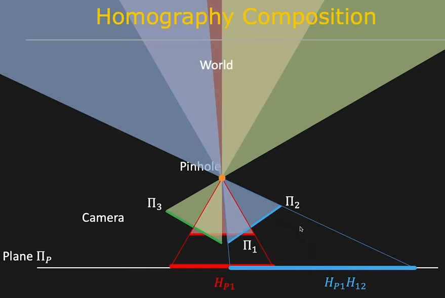
The generalized homography describes the pixel mapping from the reference plane 𝐂₁ to the plane of an arbitrary camera 𝐂ᵢ.

To apply the above derived expression 𝐇, the camera Ref-1 should always be the “world space”, and the target plane is various source camera-i.

Thus, the coordinates 𝐐’ in a source camera-i space is transformed from 𝐐 in the Ref-1 camera space as:

$$ 𝐐’ =\begin{bmatrix} 𝐑ᵢ & 𝐭ᵢ \\ 0 & 1 \end{bmatrix} \begin{bmatrix} 𝐑₁ & 𝐭₁ \\ 0 & 1 \end{bmatrix}^{-1} 𝐐 $$

The matrices product can be simplified as:

$$ \begin{bmatrix} 𝐑ᵢ & 𝐭ᵢ \\ 0 & 1 \end{bmatrix} \begin{bmatrix} 𝐑₁ & 𝐭₁ \\ 0 & 1 \end{bmatrix}^{-1} = \begin{bmatrix} 𝐑ᵢ & 𝐭ᵢ \\ 0 & 1 \end{bmatrix} \frac{1}{𝐑₁}\begin{bmatrix} 1 & -𝐭₁ \\ 0 & 𝐑₁ \end{bmatrix} = \\ \begin{bmatrix} 𝐑ᵢ & 𝐭ᵢ \\ 0 & 1 \end{bmatrix} \begin{bmatrix}𝐑₁⁻¹ & -𝐑₁⁻¹𝐭₁ \\ 0 & 1 \end{bmatrix} = \begin{bmatrix} 𝐑ᵢ𝐑₁⁻¹ & -𝐑ᵢ𝐑₁⁻¹𝐭₁+𝐭ᵢ \\ 0 & 1 \end{bmatrix} \\ $$

Therefore, the generalized relation between 𝐐’ and 𝐐 is:

$$ 𝐐’ = \tilde{𝐑}𝐐+ \tilde{𝐭} = 𝐑ᵢ𝐑₁⁻¹ 𝐐 + (-𝐑ᵢ𝐑₁⁻¹𝐭₁+𝐭ᵢ)$$

Substituting $\tilde{𝐑}$ and $\tilde{𝐭}$ into the planar homography:

$$ 𝐪 =𝐊ᵢ (𝐑ᵢ𝐑₁⁻¹ - \frac{(-𝐑ᵢ𝐑₁⁻¹𝐭₁+𝐭ᵢ) 𝐧ᵀ}{d} ) 𝐊₁⁻¹𝐩 $$

Rearrange it to align with the MVSNet paper:

$$ 𝐪 =𝐊ᵢ 𝐑ᵢ(𝐑₁⁻¹ - \frac{(-𝐑₁⁻¹𝐭₁+𝐑ᵢ⁻¹𝐭ᵢ)𝐧ᵀ}{d}) 𝐊₁⁻¹𝐩 \\ = 𝐊ᵢ 𝐑ᵢ ( 𝐈 - \frac{(-𝐑₁⁻¹𝐭₁+𝐑ᵢ⁻¹𝐭ᵢ) 𝐧ᵀ 𝐑₁}{d})𝐑₁⁻¹ 𝐊₁⁻¹𝐩 $$

The eq. (1) in MVSNet was wrong: $𝐇_i(d) = 𝐊ᵢ 𝐑ᵢ ( 𝐈 - \frac{(𝐭₁-𝐭ᵢ) 𝐧ᵀ}{d})𝐑₁ᵀ 𝐊₁ᵀ$, (issue #77)

$𝐊₁⁻¹ \neq 𝐊₁ᵀ$ since 𝐊 may not be an orthogonal matrix.
𝐑ᵢ⁻¹ and 𝐑₁ can’t be cancled.

Corresponding to MVSNet-TF code, c_left is $-𝐑₁⁻¹𝐭₁$; c_right is $-𝐑ᵢ⁻¹𝐭ᵢ$; c_relative is $-(-𝐑₁⁻¹𝐭₁+𝐑ᵢ⁻¹𝐭ᵢ)$ fronto_direction is $-𝐧ᵀ 𝐑₁$, which is R_left[2,:]. Therefore, temp_vec = tf.matmul(c_relative, fronto_direction) is $(-𝐑₁⁻¹𝐭₁+𝐑ᵢ⁻¹𝐭ᵢ) 𝐧ᵀ 𝐑₁$.

Warp An Image

(2023-12-19) Homography warps a non-rectangle to a rectangle.

(2023-02-08)

Homography matrix warps an image to another plane. In the application of image stitching, multiple images are warped to a unified plane.

The images have to be observing the common plane.

It works for stitching planar panoramas because the scene is far from the camera.
(2023-12-17) In other words, co-planar points remain co-planar after a homography transformation (matrix). For example, a point on a plane that in image-1 remains located on the plane viewed by image-2.

Two pairs of matched points will perform the same transformation: $$\begin{cases}p_1 = H p_2 \\ q_1 = H q_2 \end{cases}$$

Put differently, “a plane remains a plane in another view”, while the portion that is not on the plane will be warped.

R,T can be solved from H and K.

Demo: Warp the image to simulate the scene seen from another displaced camera (Aerial View). Refer to: OTC4 Homography說明以及小實驗-AI葵

Select 10 points to form a plane, which remains a plane in another view after transformion.

 1
 2
 3
 4
 5
 6
 7
 8
 9
10
11
12
13
14
15
16
17
18
19
20
21
22
23
24
25
26


import cv2
import numpy as np
import matplotlib.pyplot as plt
%matplotlib inline

img1 = cv2.imread("rot1.png")
pts1 = [(24, 124), (49, 124), (98, 124), (104, 124), (120, 124),
        (18, 146), (37, 146), (65, 146), (102, 146), (133, 146)]
for pt in pts1:
  cv2.circle(img1, pt, 0, (0, 0, 255))
plt.figure(figsize=(20,10))
plt.imshow(img1[:,:, ::-1])

img2 = cv2.imread("rot2.png")
pts2 = [(45, 116), (64, 120), (110, 127), (118, 128), (135, 131),
        (31, 135), (46, 137), (69, 143), (105, 150), (140, 158)]

src_points = np.array(pts1, dtype=np.float32).reshape(-1,1,2)
dst_points = np.array(pts2, dtype=np.float32).reshape(-1,1,2)
Homography, mask = cv2.findHomography(src_points, dst_points, 0, 0.0) # (3,3)

# warp img1 to the view of img2
warped1 = cv2.warpPerspective(img1, Homography, (img1.shape[1], img1.shape[0]))
plt.figure(figsize=(20,10))
plt.imshow(warped1[:,:,::-1]) # reverse
plt.imshow(img2[:,:,::-1], alpha=0.6) # overlap

Bird’s-Eye View:

1
2
3
4
5


src_trapezoid = np.float32([[1, 128], [47, 91], [120, 91], [157, 128]])
dst_rectangle = np.float32([[64, 104], [64, 64], [104, 64], [104, 104]])

homoMatrix = cv2.getPerspectiveTransform(src_trapezoid, dst_rectangle)
warped = cv2.warpPerspective(img, homoMatrix,(img.shape[1], img.shape[0]))

The image got transformed by the homography to deform the trapezoidal road lane to a rectangle displaying on the image by changing the camera pose to looking down:

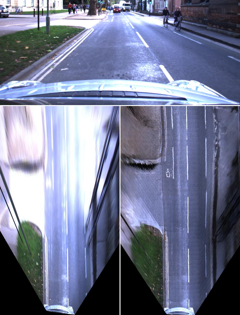
BEV is a homography, but only make sense for the ground plane. 单应性Homograph估计：从传统算法到深度学习 - 白裳的文章 - 知乎

Multi-Depth Planes

(2023-12-17)

Given camera parameters of a reference view and a source view in the world space respectively, and multiple depth planes, solve the homographies that transforming the source image into the reference camera space:

The formula used in MVSNet-tf code is: $𝐊ᵢ𝐑ᵢ ( 𝐈 - \frac{-(-𝐑₁⁻¹𝐭₁+𝐑ᵢ⁻¹𝐭ᵢ) (-𝐧ᵀ 𝐑₁)}{d})𝐑₁⁻¹𝐊₁⁻¹$ because the $-𝐧ᵀ 𝐑₁$ is the z-axis of 𝐑₁ in the world space.

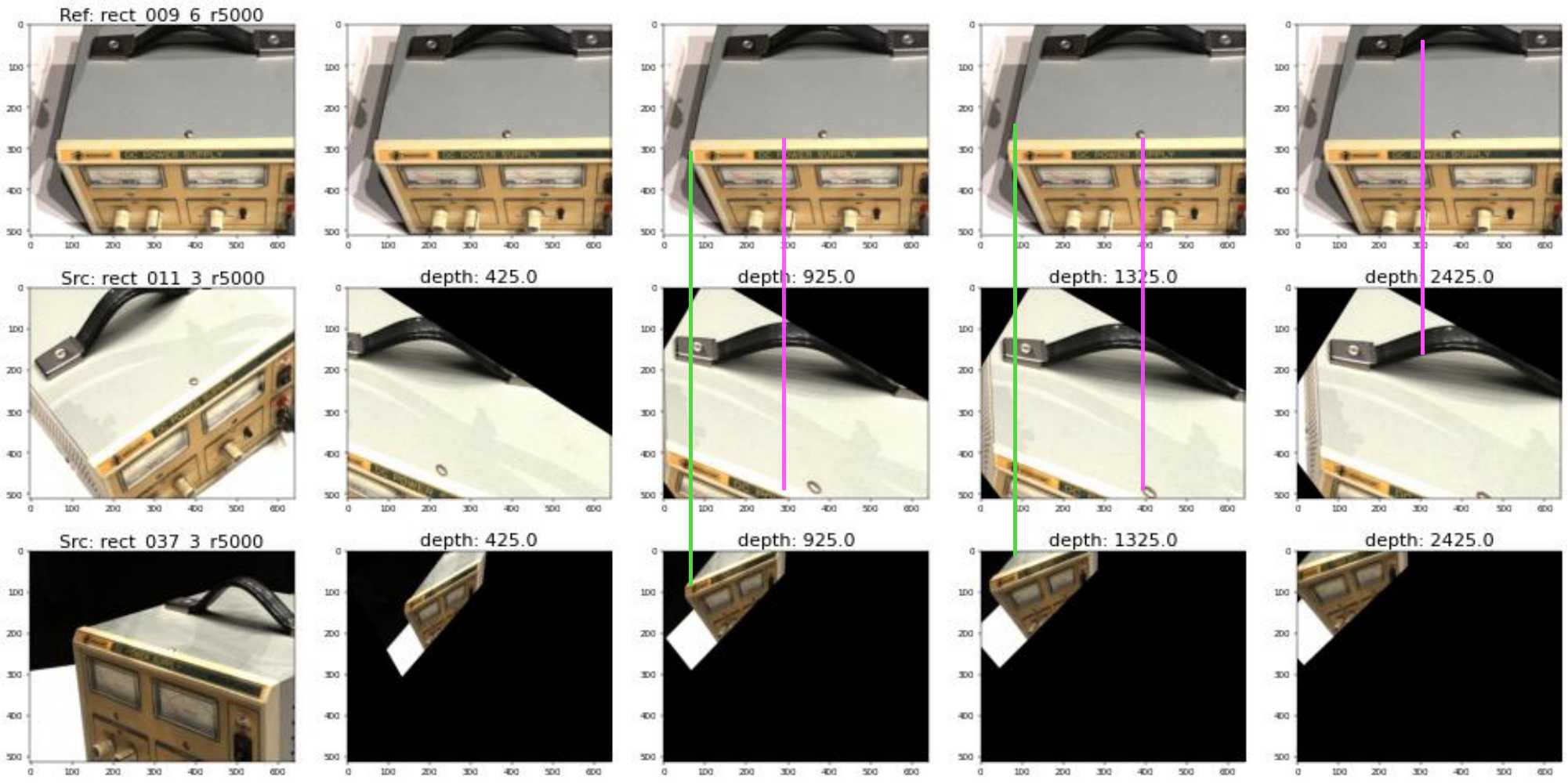
A source images is warped to the reference camera space and watching a common depth plane. Therefore, the points on the depth plane will have the same x coordinates as the points in the reference image.

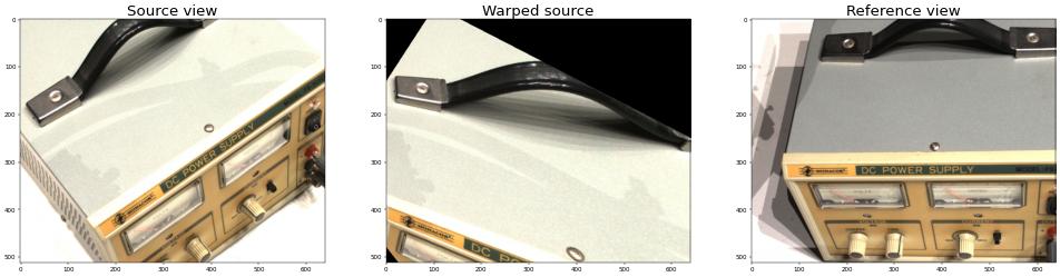
Warp by Sampling

(2023-12-18)

Sample the source image to be warped at the locations that is determined by the mapping of homography inversely from the target view to the source view. Refer to MVSNet-pytorch.

 1
 2
 3
 4
 5
 6
 7
 8
 9
10
11
12
13
14
15
16
17
18
19
20
21
22
23
24
25
26
27
28
29
30
31
32
33
34
35
36


import torch
from torchvision import transforms

h, w = ref.shape[:2]
vu = torch.cartesian_prod(torch.arange(h), torch.arange(w))
uv = torch.flip(vu, [1])  # (hw,2), As x varies, y is fixed
uv1 = torch.cat([uv, torch.ones(len(uv), 1)], dim=-1) # (hw,3)

src_KRT = torch.eye(4)
src_KRT[:3] = torch.from_numpy(K_s @ RT_s[:3, :4])
ref_KRT = torch.eye(4)
ref_KRT[:3] = torch.from_numpy(K_r @ RT_r[:3, :4])
proj = src_KRT @ torch.inverse(ref_KRT)

rot, trans = torch.split(proj, [3,1], dim=-1)   
rot_uv1 = rot[:3] @ uv1.t()  # (3, hw)
d = 425.0 + 1.06*2.5 * torch.arange(192).view(1,-1,1)  #(1, 192, 1)
rot_uvd = rot_uv1.unsqueeze(1).expand(-1, 192,-1) * d  #(3, 192, hw)
pix_proj = rot_uvd + trans[:3].unsqueeze(1).expand(-1, 192, -1) # (3, 192, hw)

u_src = 2*(pix_proj[0] / pix_proj[2])/(w-1)-1
v_src = 2*(pix_proj[1] / pix_proj[2])/(h-1)-1
uv_src = torch.stack([u_src, v_src], dim=-1)    # (192, hw, 2)
uv_src_d1 = uv_src[-1]  # plane at the furthest depth
sampled = torch.nn.functional.grid_sample(
          transforms.ToTensor()(src).unsqueeze(0),  # (1,3,512,640)
          uv_src_d1.view(1, h, w, 2), mode='nearest')
sampled_scaled = torch.tensor(sampled[0] * 255, dtype=int)  # (3, 512, 640)

fig, ax = plt.subplots(1,3, figsize=(30,15))
ax[0].imshow(src[:,:,::-1]) # (512, 640, 3)
ax[0].set_title("Source view")
ax[1].imshow(sampled_scaled.permute(1,2,0).numpy()[:,:,::-1])
ax[1].set_title("Warped source")
ax[2].imshow(ref[:,:,::-1])
ax[2].set_title("Reference view")

The result is almost the same as the one yielded by opencv:

4 Co-planar Points

(2022-12-03)

Homography matrix builds the relatioship between 2 images to make the pixels corresponding to the same 3D points overlap ³ based on the projection from the common 3D point to different image planes.

In following example, two cameras look at a flat plane. And they both observe the points located on that flat plane.

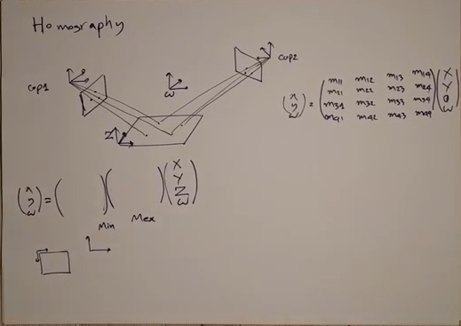
Then, the matching pixels on the two camera planes can be connected by the chain: img1 ➔ plane0 ➔ img2.

When a 3D world point is projected to 2D camera plane, the coordinates transformation consists of two matrix: extrinsic matrix [R|T] transforming the coordinate system, and the intrinsic matrix [K] projecting the 3D point to a 2D pixel, that is:

$$ \begin{bmatrix} u\\ v\\ 1\\ 1 \end{bmatrix} = \begin{bmatrix} f/dₓ & 0 & cₓ & 0 \\ 0 & f/d_y & c_y & 0 \\ 0 & 0 & 1 & 0 \\ 0 & 0 & 0 &1 \end{bmatrix} \begin{bmatrix} r₁₁ & r₁₂ & r₁₃ & t₁ \\ r₂₁ & r₂₂ & r₂₃ & t₂ \\ r₃₁ & r₃₂ & r₃₃ & t₃ \\ 0 & 0 & 0 & 1 \end{bmatrix} \begin{bmatrix} X \\ Y \\ Z \\ W \end{bmatrix} $$

where the W is the homogeneous coordinate for accommodating the translation vector $[^{^{t₁}_{t₂}} _{^{t₃}_{1}}]$ in the extrinsic matrix.

Omit z because all points on the plane have z=0.

Given $[^{_{x₁}}_{^{y₁}_{w₁}}]$ = H₁₀ $[^{_{x₀}}_{^{y₀}_{w₀}}]$, then there is $$\rm [^{_{x₂}}_{^{y₂}_{w₂}}] = H₂₀ H₁₀⁻¹[^{_{x₁}}_{^{y₁}_{w₁}}]$$, where H₂₀ H₁₀⁻¹ is the homograhpy matrix H₃ₓ₃. It represents the mapping between the pair of points: (x₁,y₁,w₁) and (x₂,y₂,w₂).

$$ \begin{bmatrix} x₂\\ y₂\\ w₂ \end{bmatrix} = \begin{bmatrix} H₁₁ & H₁₂ & H₁₃ \\ H₂₁ & H₂₂ & H₂₃ \\ H₃₁ & H₃₂ & H₃₃ \\ \end{bmatrix} \begin{bmatrix} x₁\\ y₁\\ w₁ \end{bmatrix} $$

Expand the above equation, there are 2 equations (with considering x₂’=x₂/w₂, y₂’=y₂/w₂, such that w = 1):

$$\begin{cases} x₂’ = \frac{x₂}{w₂} = \frac{H₁₁x₁ + H₁₂y₁ + H₁₃w₁}{H₃₁x₁ + H₃₂y₁ + H₃₃w₁} \\ y₂’ = \frac{y₂}{w₂} = \frac{H₂₁x₁ + H₂₂y₁ + H₂₃w₁}{H₃₁x₁ + H₃₂y₁ + H₃₃w₁}\end{cases} \\ ⇓ \\ \rm\{^{x₂’H₃₁x₁ + x₂’H₃₂y₁ + x₂’H₃₃w₁ - H₁₁x₁ - H₁₂y₁ - H₁₃w₁ = 0} _{y₂’H₃₁x₁ + y₂’H₃₂y₁ + y₂’H₃₃w₁ - H₂₁x₁ - H₂₂y₁ - H₂₃w₁ = 0} $$

The last element H₃₃ is determined when other elements are set, so the degree of freedom for this matrix is 8.

Therefore, the homography matrix can be solved from 4 pairs of matching points: (x₁,y₁)-(x₂,y₂); (x₃,y₃)-(x₄,y₄); (x₅,y₅)-(x₆,y₆); (x₇,y₇)-(x₈,y₈).

After reformalizing the equation system to a matrix form, the sigular value decomposition can be applied.

$$\rm{ [^{^{^{-x₁\; -y₁\; -w₁\; 0\quad 0\quad 0\quad x₂’x₁\quad x₂’y₁\quad x₂’w₁} _{0\quad 0\quad 0\quad -x₁\; -y₁\; -w₁\; y₂’x₁\quad y₂’y₁\quad y₂’w₁}} _{^{-x₃\; -y₃\; -w₃\; 0\quad 0\quad 0\quad x₄’x₃\quad x₄’y₃\quad x₄’w₃} _{0\quad 0\quad 0\quad -x₃\; -y₃\; -w₃\; y₄’x₃\quad y₄’y₃\quad y₄’w₃}}} _{^{^{pair3-1}_{pair3-2}} _{^{pair4-1}_{pair4-2}}}] \ [^{^{^{H₁₁}_{H₁₂}} _{^{H₁₃}_{H₂₁}}} _{^{^{H₂₂}_{H₂₃}} _{^{H₃₁}_{^{H₃₂}_{H₃₃}}}}] = 0 } $$

Solution

This is a homogeneous linear system 𝐀𝐡=0, so its solution has 2 cases:

If the number of non-zero rows of the coefficients matrix 𝐀 after Gaussian elimination is less than the number of unknowns of 𝐡, i.e., (rank(𝐀) < #h), there is only the zero solution;
Or infinitely many non-zero solution, but only the solution satisfying constraints of magnitude is selected.

If 𝐀 is invertible (square matrix & rank(𝐀) = #col), then 𝐡=𝐀⁻¹⋅0 = 0 ???

Otherwise, if 𝐀 is not invertible, there would be inifinetly many non-zero solutions. So the optimal solution should be approached by minimizing the error $$J = ½‖𝐀𝐡-0‖²$$ Therefore, the least-square solution is when the derivative

$$ ∂J/∂𝐡 = 0 \\ ⇒ 𝐀ᵀ(𝐀𝐡-0) = 0\\ ⇒ 𝐀ᵀ𝐀𝐡-𝐀ᵀ⋅0 = 0 $$

If 𝐀ᵀ𝐀 is invertible, the optimal 𝐡=(𝐀ᵀ𝐀)⁻¹𝐀ᵀ⋅0 = 0 ???, where the (𝐀ᵀ𝐀)⁻¹𝐀ᵀ is the pseudo-inverse matrix.

Use all the matching pints to compute a robust H, even though 4 pairs are enough to solve the 8 unkowns (An element is 1 after scaling the matrix by it).
1. Constrained Least Squares. Solve for 𝐡: A𝐡=0, such that ‖𝐡‖²=1.
  Define least squares problem: min_𝐡 ‖A𝐡‖², such that ‖𝐡‖²=1. We know that: ‖A𝐡‖² = (A𝐡)ᵀ(A𝐡) = 𝐡ᵀAᵀA𝐡, and ‖𝐡‖²= 𝐡ᵀ𝐡 =1. So the problem is: minₕ(𝐡ᵀAᵀA𝐡), such that 𝐡ᵀ𝐡 =1.
  
  Define Loss function L(𝐡,λ): L(𝐡,λ)= 𝐡ᵀAᵀA𝐡 - λ(𝐡ᵀ𝐡 -1). And take derivatives of L(𝐡,λ) w.r.t. 𝐡: 2AᵀA𝐡 - 2λ𝐡 =0. It’s the classical eigenvalue problem: AᵀA𝐡 = λ𝐡.
2. SVD.
  Find the eigenvalue and eigenvectors of the matrix AᵀA. 𝐡 is he eighenvector with the smallest eigenvalue λ.

First Principles of CV-Dr.Shree;

Misc

(2023-12-07) Epipolar geometry requires translation between cameras, whereas homography doesn’t. homography - Carleton University